Which permutation test implementation in R to use instead of t-tests (paired and non-paired)?

Question

I have data from an experiment that I analyzed using t-tests. The dependent variable is interval scaled and the data are either unpaired (i.e., 2 groups) or paired (i.e., within-subjects). E.g. (within subjects):

x1 <- c(99, 99.5, 65, 100, 99, 99.5, 99, 99.5, 99.5, 57, 100, 99.5, 
        99.5, 99, 99, 99.5, 89.5, 99.5, 100, 99.5)
y1 <- c(99, 99.5, 99.5, 0, 50, 100, 99.5, 99.5, 0, 99.5, 99.5, 90, 
        80, 0, 99, 0, 74.5, 0, 100, 49.5)

However, the data are not normal so one reviewer asked us to use something other than the t-test. However, as one can easily see, the data are not only not normally distributed, but the distributions are not equal between conditions:

Therefore, the usual nonparametric tests, the Mann-Whitney-U-Test (unpaired) and the Wilcoxon Test (paired), cannot be used as they require equal distributions between conditions. Hence, I decided that some resampling or permutation test would be best.

Now, I am looking for an R implementation of a permutation-based equivalent of the t-test, or any other advice on what to do with the data.

I know that there are some R-packages that can do this for me (e.g., coin, perm, exactRankTest, etc.), but I don't know which one to pick. So, if somebody with some experience using these tests could give me a kick-start, that would be ubercool.

UPDATE: It would be ideal if you could provide an example of how to report the results from this test.

Answer 1

It shouldn't matter that much since the test statistic will always be the difference in means (or something equivalent). Small differences can come from the implementation of Monte-Carlo methods. Trying the three packages with your data with a one-sided test for two independent variables:

DV <- c(x1, y1)
IV <- factor(rep(c("A", "B"), c(length(x1), length(y1))))
library(coin)                    # for oneway_test(), pvalue()
pvalue(oneway_test(DV ~ IV, alternative="greater", 
                   distribution=approximate(B=9999)))
[1] 0.00330033

library(perm)                    # for permTS()
permTS(DV ~ IV, alternative="greater", method="exact.mc", 
       control=permControl(nmc=10^4-1))$p.value
[1] 0.003

library(exactRankTests)          # for perm.test()
perm.test(DV ~ IV, paired=FALSE, alternative="greater", exact=TRUE)$p.value
[1] 0.003171822

To check the exact p-value with a manual calculation of all permutations, I'll restrict the data to the first 9 values.

x1 <- x1[1:9]
y1 <- y1[1:9]
DV <- c(x1, y1)
IV <- factor(rep(c("A", "B"), c(length(x1), length(y1))))
pvalue(oneway_test(DV ~ IV, alternative="greater", distribution="exact"))
[1] 0.0945907

permTS(DV ~ IV, alternative="greater", exact=TRUE)$p.value
[1] 0.0945907

# perm.test() gives different result due to rounding of input values
perm.test(DV ~ IV, paired=FALSE, alternative="greater", exact=TRUE)$p.value
[1] 0.1029412

# manual exact permutation test
idx  <- seq(along=DV)                 # indices to permute
idxA <- combn(idx, length(x1))        # all possibilities for different groups

# function to calculate difference in group means given index vector for group A
getDiffM <- function(x) { mean(DV[x]) - mean(DV[!(idx %in% x)]) }
resDM    <- apply(idxA, 2, getDiffM)  # difference in means for all permutations
diffM    <- mean(x1) - mean(y1)       # empirical differencen in group means

# p-value: proportion of group means at least as extreme as observed one
(pVal <- sum(resDM >= diffM) / length(resDM))
[1] 0.0945907

coin and exactRankTests are both from the same author, but coin seems to be more general and extensive - also in terms of documentation. exactRankTests is not actively developed anymore. I'd therefore choose coin (also because of informative functions like support()), unless you don't like to deal with S4 objects.

EDIT: for two dependent variables, the syntax is

id <- factor(rep(1:length(x1), 2))    # factor for participant
pvalue(oneway_test(DV ~ IV | id, alternative="greater",
                   distribution=approximate(B=9999)))
[1] 0.00810081

Answer 2

A few comments are, I believe, in order.

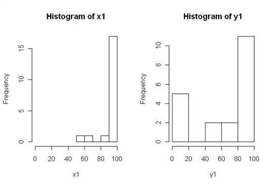
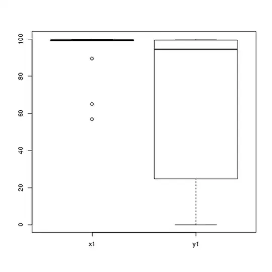
1) I would encourage you to try multiple visual displays of your data, because they can capture things that are lost by (graphs like) histograms, and I also strongly recommend that you plot on side-by-side axes. In this case, I do not believe the histograms do a very good job of communicating the salient features of your data. For example, take a look at side-by-side boxplots:

boxplot(x1, y1, names = c("x1", "y1"))

Or even side-by-side stripcharts:

stripchart(c(x1,y1) ~ rep(1:2, each = 20), method = "jitter", group.names = c("x1","y1"), xlab = "")

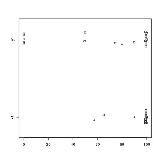
Look at the centers, spreads, and shapes of these! About three-quarters of the $x1$ data fall well above the median of the $y1$ data. The spread of $x1$ is tiny, while the spread of $y1$ is huge. Both $x1$ and $y1$ are highly left-skewed, but in different ways. For example, $y1$ has five (!) repeated values of zero.

2) You didn't explain in much detail where your data come from, nor how they were measured, but this information is very important when it comes time to select a statistical procedure. Are your two samples above independent? Are there any reasons to believe that the marginal distributions of the two samples should be the same (except for a difference in location, for example)? What were the considerations prior to the study that led you to look for evidence of a difference between the two groups?

3) The t-test is not appropriate for these data because the marginal distributions are markedly non-normal, with extreme values in both samples. If you like, you could appeal to the CLT (due to your moderately-sized sample) to use a $z$-test (which would be similar to a z-test for large samples), but given the skewness (in both variables) of your data I would not judge such an appeal very convincing. Sure, you can use it anyway to calculate a $p$-value, but what does that do for you? If the assumptions aren't satisfied then a $p$-value is just a statistic; it doesn't tell what you (presumably) want to know: whether there is evidence that the two samples come from different distributions.

4) A permutation test would also be inappropriate for these data. The single and often-overlooked assumption for permutation tests is that the two samples are exchangeable under the null hypothesis. That would mean that they have identical marginal distributions (under the null). But you are in trouble, because the graphs suggest that the distributions differ both in location and scale (and shape, too). So, you can't (validly) test for a difference in location because the scales are different, and you can't (validly) test for a difference in scale because the locations are different. Oops. Again, you can do the test anyway and get a $p$-value, but so what? What have you really accomplished?

5) In my opinion, these data are a perfect (?) example that a well chosen picture is worth 1000 hypothesis tests. We don't need statistics to tell the difference between a pencil and a barn. The appropriate statement in my view for these data would be "These data exhibit marked differences with respect to location, scale, and shape." You could follow up with (robust) descriptive statistics for each of those to quantify the differences, and explain what the differences mean in the context of your original study.

6) Your reviewer is probably (and sadly) going to insist on some sort of $p$-value as a precondition to publication. Sigh! If it were me, given the differences with respect to everything I would probably use a nonparametric Kolmogorov-Smirnov test to spit out a $p$-value that demonstrates that the distributions are different, and then proceed with descriptive statistics as above. You would need to add some noise to the two samples to get rid of ties. (And of course, this all assumes that your samples are independent which you didn't state explicitly.)

This answer is a lot longer than I originally intended it to be. Sorry about that.

Answer 3

As this question did pop up again, I may add another answer inspired by a recent blog post via R-Bloggers from Robert Kabacoff, the author of Quick-R and R in Action using the lmPerm package.

However, this methods produces sharply contrasting (and very unstable) results to the one produced by the coin package in the answer of @caracakl (the p-value of the within-subjects analysis is 0.008). The analysis takes the data preparation from @caracal's answer as well:

x1 <- c(99, 99.5, 65, 100, 99, 99.5, 99, 99.5, 99.5, 57, 100, 99.5, 
        99.5, 99, 99, 99.5, 89.5, 99.5, 100, 99.5)
y1 <- c(99, 99.5, 99.5, 0, 50, 100, 99.5, 99.5, 0, 99.5, 99.5, 90, 
        80, 0, 99, 0, 74.5, 0, 100, 49.5)

DV <- c(x1, y1)
IV <- factor(rep(c("A", "B"), c(length(x1), length(y1))))
id <- factor(rep(1:length(x1), 2)) 

library(lmPerm)

summary(aovp( DV ~ IV + Error(id)))

produces:

> summary(aovp( DV ~ IV + Error(id)))
[1] "Settings:  unique SS "

Error: id
Component 1 :
          Df R Sum Sq R Mean Sq
Residuals 19    15946       839


Error: Within
Component 1 :
          Df R Sum Sq R Mean Sq Iter Pr(Prob)  
IV         1     7924      7924 1004    0.091 .
Residuals 19    21124      1112                
---
Signif. codes:  0 ‘***’ 0.001 ‘**’ 0.01 ‘*’ 0.05 ‘.’ 0.1 ‘ ’ 1 

If you run this multiple times, the p-values jumps around between ~.05 and ~.1.

Although it is an answer to the question let me allow to pose a question at the end (I can move this to a new question if desired):
Any ideas of why this analysis is so unstable and does produce a so diverging p-values to the coin analysis? Did I do something wrong?

Answer 4

My comments are not about implementation of the permutation test but about the more general issues raised by these data and the discussion of it, in particular the post by G. Jay Kerns.

The two distributions actually look quite similar to me EXCEPT for the group of 0s in Y1, which are much different from the other observations in that sample (next smallest is about 50 on the 0-100 scale) as well as all those in X1. I would first investigate whether there was anything different about those observations.

Second, assuming those 0s do belong in the analysis, saying the permutation test isn't valid because the distributions appear to differ begs the question. If the null were true (distributions are identical), could you (with reasonable probability) get distributions looking as different as these two? Answering that's the whole point of the test, isn't it? Maybe in this case some will consider the answer obvious without running the test, but with these smallish, peculiar distributions, I don't think I would.

Answer 5

Are these scores proportions? If so, you certainly shouldn't be using a gaussian parametric test, and while you could go ahead with a non-parametric approach like a permutation test or bootstrap of the means, I'd suggest that you'll get more statistical power by employing a suitable non-gaussian parametric approach. Specifically, any time you can compute a proportion measure within a unit of interest (ex. participant in an experiment), you can and probably should use a mixed effects model that specifies observations with binomially distributed error. See Dixon 2004.

Answer 6

Just adding another approach, ezPerm of ez package:

> # preparing the data
> DV <- c(x1, y1)
> IV <- factor(rep(c("A", "B"), c(length(x1), length(y1))))
> id <- factor(rep(1:length(x1), 2))
> df <- data.frame(id=id,DV=DV,IV=IV)
>
> library(ez)
> ezPerm( data = df, dv = DV, wid = id, within = IV, perms = 1000)
|=========================|100%              Completed after 17 s 
  Effect     p p<.05
1     IV 0.016     *

This seems to be consistent to the oneway_test of the coin package:

> library(coin)
> pvalue(oneway_test(DV ~ IV | id,  distribution=approximate(B=999999)))
[1] 0.01608002
99 percent confidence interval:
 0.01575782 0.01640682

However, notice that this is not the same example provided by @caracal. In his example, he includes alternative="greater", therefore the difference in p-values ~0.008 vs ~0.016.

The aovp package suggested in one of the answers produce suspiciously lower p-values, and runs suspiciously fast even when I try high values for the Iter, Ca and maxIter arguments:

library(lmPerm)
summary(aovp(DV ~ IV + Error(id/IV), data=df,  maxIter = 1000000000))
summary(aovp(DV ~ IV + Error(id/IV), data=df,  Iter = 1000000000))
summary(aovp(DV ~ IV + Error(id/IV), data=df,  Ca = 0.00000000001))

That said, the arguments seems to be slightly reducing the variations of p-values from ~.03 and ~.1 (I got a bigger range thant the reported by @Henrik), to 0.03 and 0.07.