0

Follow the very useful answers from Peter Flom, Wayne and many others. I have now started using R and it gives me a feeling of python :)

The results are below but I am not sure how should I go from here ? The density certain looks much better after log transformation. Can you please shed some light on how to do further analysis ?

Thanks a lot.

R - Results below:

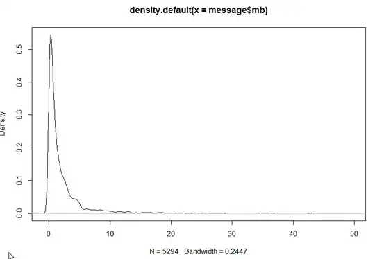
plot (density (messages$length)) enter image description here

plot (density (log (messages$length))) enter image description here summary (messages)

> summary(message$mb)
    Min.  1st Qu.   Median     Mean  3rd Qu.     Max. 
 0.00665  0.32610  0.88450  2.08500  2.35000 49.13000 

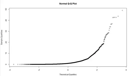
qqnorm (messages$length) enter image description here

=====================================================================

EDIT: Thanks all all the answering !

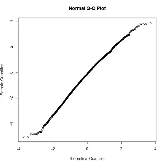
I have tried the qqnorm with log(x) and it looks like a straight line ! Does this mean my data is pretty much following a Log-normal distribution ?

qqnorm (log(messages$length)):

enter image description here

Also I have tried to fit my data with a log-normal and below is the result.

fitdistr(message$mb, densfun="log-normal") meanlog sdlog
-0.19019347 1.45795269 ( 0.02003787) ( 0.01416891)

Does this mean anything ?

RoundPi
  • 145
  • 1
  • 1
  • 6
  • 1
    The log-transformed data look quite normal. You could try to use the `fitdistr` function from the `MASS` package. On your untransformed data, you could try to fit a log-normal distribution: `fitdistr(messages$length, densfun="log-normal")`. [This post](http://stats.stackexchange.com/questions/58220/what-distribution-does-my-data-follow) might provide some further imputs. – COOLSerdash May 23 '13 at 15:56
  • 3
    You can push the logarithms through `qqnorm()` too. If there is systematic curvature, lognormal is not quite right, although that doesn't mean that there is a much better candidate. Gamma might be another one to try. My wild guess from the density plot is that lognormal will work better than the gamma. – Nick Cox May 23 '13 at 16:55
  • @NickCox, do you mean log then qqnorm ? – RoundPi May 23 '13 at 22:18
  • 2
    Yes. I am only a very occasional R user, but you can exploit the definition of lognormal, that if x is lognormal then log x is normal, and `qqnorm()` applied to that should show a straight line. – Nick Cox May 23 '13 at 22:28
  • @NickCox, Thanks for the explanation and I have updated it! – RoundPi May 24 '13 at 11:08
  • @COOLSerdash, I have also tried fitdistr but I am not sure if the result means much ? – RoundPi May 24 '13 at 11:09
  • 1
    @Gob00st Thanks for updating your question. I would suggest that you use the `qqPlot` function from the `car` package. Then you could either put `qqPlot(messages$length, distribution="lnorm")` or `qqPlot(log(messages$length), distribution="norm")` to fit QQ-plot on the original scale or on the log-scale. The output from `fitdistr` are the mean and sd of your distribution on the log scale. – COOLSerdash May 24 '13 at 11:19
  • @COOLSerdash, I have tried to use car package but it seems it's not within the latest R installation. Is there a way to calculate the probability for message size of 45M from the density or from the raw data within R? – RoundPi May 24 '13 at 12:13
  • 1
    @Gob00st Have you tried to install the package (`install.packages("car")`)? That works for me. If you assume that your data follow a log-normal distribution with a mean of -0.19 and a sd of 1.458 on the log scale, you can use the CDF of the normal distribution to calculate the probability that a message exceeds 45M: `1-pnorm(log(45), mean=-0.19019347, sd=1.45795269)` This gives a probability of 0.0031. – COOLSerdash May 24 '13 at 12:22
  • @COOLSerdash: thanks for the quick reply! I will give it a go after lunch. Also I am not sure at which point can I assume it's a log-normal. Also is it normal to have a negative mean for log normal ? My data is based on actual message size and it really shouldn't go to 0 or below. – RoundPi May 24 '13 at 12:45
  • 1
    @Gob00st From what I've seen of your data, they seem compatible with a log-normal distribution. The negative mean is on the *log scale*. This is the mean of `log(messages$length)`. The mean of your data on the original scale would be: $\exp(\mu + \sigma^2/2)$, so around 2.39 (with $\mu=-0.19$ and $\sigma^{2}=1.458^{2}=2.126$. The variance would be $[\exp(\sigma^{2}) - 1]\cdot \exp(2\mu + \sigma^{2})=42.257$. – COOLSerdash May 24 '13 at 12:52
  • @COOLSerdash: Thanks!!! Nicely explained !!! How silly I was! – RoundPi May 24 '13 at 13:05

1 Answers1

2

I want to quickly summarize my comments for your convenience. From what I've seen of your data, they seem compatible with a log-normal distribution with a mean and standard deviation on the log scale of $\mu=-0.19$ and $\sigma=1.458$, respectively. The density plot of your log-transformed data is not perfectly symmetrical, it has a small negative skew. "On the log scale" means that the mean and standard deviation given are those corresponding to the log-transformed data - which should follow a normal distribution then. The mean on your original scale would be $\exp(\mu + \sigma^{2}/2)$ and the standard deviation $\sqrt{\left[\exp(\sigma^{2})-1 \right]\cdot \exp(2\mu + \sigma^{2})}$, or numerically: $2.39$ and $6.50$. The mode (the peak of your distribution) on the original scale would be $\exp(\mu - \sigma^{2})=0.099$.

The probability that a message exceeds a size of $a$ can be calculated as follows:

  • On the log scale using the CDF of the normal distribution: pnorm(log(a), mean=-0.19019347, sd=1.45795269, lower.tail=FALSE)
  • On the original scale using the CDF of the log-normal distribution: plnorm(a, meanlog=-0.19019347, sdlog=1.45795269, lower.tail=FALSE)
COOLSerdash
  • 25,317
  • 8
  • 73
  • 123