The question calls for choosing an experimental design and selecting a sample size sufficiently large to estimate the slope $\beta_1$ to within a desired level of precision.
Let $n$ be the number of observations needed and suppose an optimal solution calls for setting the explanatory variable (hydration) to values $x_1, x_2, \ldots, x_n$ (which need not be distinct). We need to find the minimal number of such values as well as what they should be set to.
In the model let the unknown variance of the disturbance terms $\varepsilon$ be $\sigma^2.$ The variance-covariance matrix of the least squares coefficient estimates $(\hat\beta_0, \hat\beta_1)$ is then
$$\pmatrix{\operatorname{Var}(\hat\beta_0) &\operatorname{Cov}(\hat\beta_0,\hat\beta_1) \\ \operatorname{Cov}(\hat\beta_1,\hat\beta_0) & \operatorname{Var}(\hat\beta_1)} = \operatorname{Var}(\hat\beta_0,\hat\beta_1) =\sigma^2\left(X^\prime X\right)^{-1}\tag{1}$$
where $X$ is the "design matrix" created by stacking the vectors $(1,x_1), \ldots, (1,x_n)$ into an $n\times 2$ array. Thus,
$$X^\prime X = \pmatrix{1&1&\cdots&1\\x_1&x_2&\cdots&x_n}\pmatrix{1&x_1\\1&x_2\\\vdots&\vdots\\1&x_n}= \pmatrix{n & S_x \\ S_x & S_{xx}}$$
where $S_x$ is the sum of the $x_i$ and $S_{xx}$ is the sum of their squares. Assuming not all the $x_i$ are equal, this matrix is invertible with inverse
$$\left(X^\prime X\right)^{-1} = \frac{1}{nS_{xx} - S_x^2} \pmatrix{S_{xx} & -S_x \\ -S_x & n},$$
from which we read off the estimation variance from the bottom right entries of $(1)$ as
$$\operatorname{Var}(\hat\beta_1) = \frac{n\sigma^2}{nS_{xx} - S_x^2}.\tag{2}$$
Given any sample size $n,$ we must choose $(x_i)$ to maximize the denominator of $(2).$ Equivalently, because $1/n^2$ times the denominator is the (population) variance of $(x_i),$ we seek to maximize that variance. When those values are constrained to an interval $[A,B],$ it is well known that
this variance is maximized by splitting the $x_i$ into two parts that are as equal in size as possible and setting one part to $A$ and the other to $B.$
This leads to two formulas for the variance--one for even $n$ and the other for odd $n$--but for this analysis it will suffice to use the one for even $n$ because it so closely approximates the one for odd $n:$ namely, the maximal variance is $(B-A)^2/4.$ From (2) we thus obtain
$$\operatorname{Var}(\hat\beta_1) \ge \frac{4n\sigma^2}{n^2(B-A)^2}.$$
Its square root is the standard error of estimate, which simplifies to
$$\operatorname{SE}(\hat\beta_1) \ge \frac{2\sigma}{(B-A)\sqrt{n}}.\tag{3}$$
Confidence intervals are obtained by moving some multiple $z(\alpha)$ (depending on the confidence level $1-\alpha$) of the standard error to either side of $\hat\beta_1.$ Consequently, given an upper threshold $W$ for the width of the confidence interval, $n$ must be large enough to make $2z$ times $(3)$ no greater than $W.$ Solving,
$$n \ge \frac{16 z(\alpha)^2\sigma^2}{W^2(B-A)^2}.$$
That's as far as we can take the answer with the given information. In practice, you don't know $\sigma:$ it reflects the variability of the response ("volume") around the linear model. Usually you have to guess it, either using previous experience, a search of literature, or true guessing. A good approach is to underestimate $n,$ perform the experiment, use the results to obtain a better estimate of $\sigma,$ re-estimate $n$ (which will almost always be larger), and then obtain the requisite number of additional observations.
There are many subtle issues. A full discussion requires a textbook on experimental design. Some of them are
This solution is unable to distinguish random variation from nonlinearity. One consequence of this is that in the presence of important curvature, a different design (involving intermediate values of $x_i$ in the interior of the interval $[A,B]$) could require far fewer observations because the associated value of $\sigma$ might be much smaller.
Technically, $Z(\alpha)$ depends on $n,$ too: it ought to be derived from a Student $t$ distribution. This problem can be overcome by first deriving it from a standard Normal distribution, computing an initial solution for $n,$ then using $n-2$ as the degrees of freedom in the Student $t$ distribution. Re-estimate $n.$ This process will converge within a few iterations to the optimal $n.$
Ultimately, the least squares procedure will estimate $\sigma.$ This estimate won't be quite the same as the true value of $\sigma.$
There is no assurance, after the full experiment is done, that the width of the confidence interval will be less than the threshold $W:$ results will vary and so will this width.
Naive and overoptimistic specifications of the confidence level $1-\alpha$ often lead to astronomically large requirements for the sample size $n.$ Almost always, one has to give up a little confidence or a little precision in order to make the sample size practicable.
Other criteria for optimal design can be considered. The one used here is both C-optimal and D-optimal. Solutions for other (related) forms of optimality can be developed using the same techniques illustrated in $(1),$ $(2),$ and $(3)$ above.
Finally, as an example of how to apply this solution, suppose (as in the question) that the interval is $[A,B]=[55,85],$ that the confidence is to be $95\%$ ($\alpha=0.05$), $\sigma=1,$ and the maximum width of a CI for $\beta_1$ is to be $0.1.$
The initial value of $Z(\alpha)$ is the lower $\alpha/2=0.025$ quantile of the standard Normal distribution, $-1.96.$ The smallest integer greater than
$$\frac{16(-1.96)^2(1)^2}{(0.1)^2(85-55)^2} \approx 6.8$$
is $7.$ The lower $0.025$ quantile of the Student $t$ distribution with $7-2=5$ degrees of freedom is $-2.57.$ Using this instead of the previous value of $Z$ multiplies the estimate by $((-2.57)/(-1.96))^2 \approx 1.7,$ giving a new sample size estimate of $n=12.$ Two more iterations bounce down to $9$ and then stop at $n=10.$
Accordingly, I set five values of $x$ to $A=55$ and five to $B=85.$ In five thousand independent simulations, I created random Normal responses according to a linear model with $\sigma=1,$ fit the model with least squares, and recorded the width of the confidence interval for $\beta_1.$ Here is a summary of those results, with the mean width shown as a red dotted line.
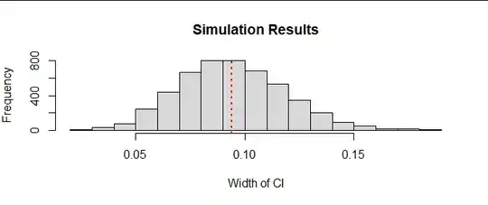
Slightly more than half the time, the width met the target of $0.1.$ (NB: the CI widths were established using least-squares estimates of $\sigma.$) The width rarely was hugely greater than the target. (The variability of the widths depends on $n$ as well as the sample design.) A quick simulation like this can help you appreciate what you might encounter in the actual experiment and might prompt you to modify your solution before you begin experimenting.
