First we have to have made a good assumption. That is, if we are assuming linearity, that actually has to be correct for the rest of the answer to be correct as well. Assuming it is correct then for a given homoscedastic noise variance, the range of $x_i$ should be chosen to be as large or broad as possible. That means that if the range of x-values is only twice, we are more likely to get insignificant slopes and intercepts than if we have a range of 10 times from minimum to maximum x-values, and 100 times would be even better, and that goes for both the slope and intercept confidence intervals.
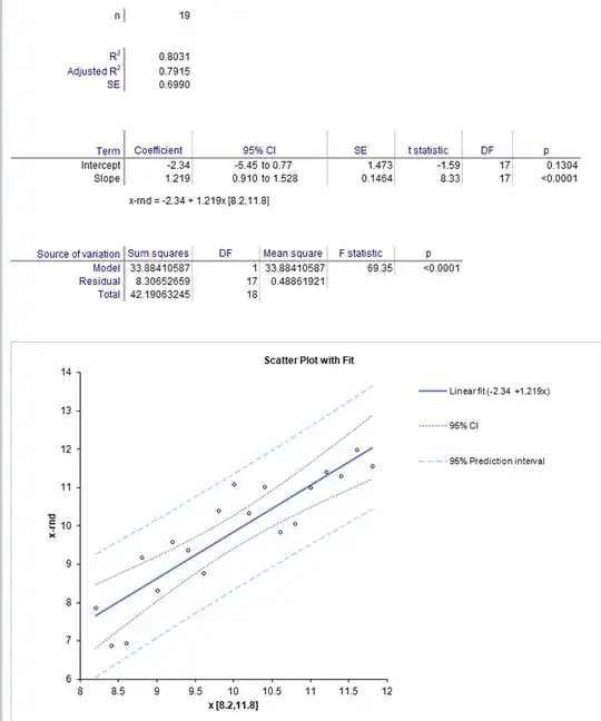
Below is an example in two cases. In the first case, we have $n=19$ x-values from $[8.2,11.8]$
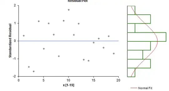
And, in the second case $n=19$ x-values from $[1,19]$
The random probabilities are identical in each case, and the number of points is identical. The random probabilities were used to generate $\mathcal{N}(0,1)$ which identical actual residuals were added to x-values to make y=x+error.
Notice that in the first case, R$^2$ is only 0.80, the 95% confidence intervals are from -5.45 to 0.770 for intercept, and 0.910 to 1.528 for slope.
In the second case, R$^2$ is 0.99, the 95% confidence intervals are from -1.29 to 0.117 for intercept, and 0.982 to 1.106 for slope.
That is, the 95% confidence interval for a 5 fold increase in x-value range has decreased by exactly 5 times for slope, and by 4.411 times for intercept.
Here are the residuals for the first case:
 And now for the second case:
 Note that the only thing that has changed is the scale of the x-axis.
Now, if the model is wrong, there is no such guarantee, for example if we are using a linear to approximate a quadratic distributed random variate, a larger range of x-values could produce less certainty in the linear slope and intercept. Also, if the noise is not homoscedastic, then transformation of variables should be undertaken first, and then an appropriate model for the transformed variables should be selected. Often, when the transformation is more homoscedastic, the model is better behaved in terms of goodness of fit, as the data may then be better linearized, or not, depending on the context.
Here is an example of the effect of reducing heteroscedasticity from the literature: An improved method for determining renal sufficiency using volume of distribution and weight from bolus 99mTc-DTPA, two blood sample, paediatric data