as I am stepping into forecasting with ARIMA models, I am trying to understand how I can improve a forecast based on ARIMA fit with seasonality and drift.
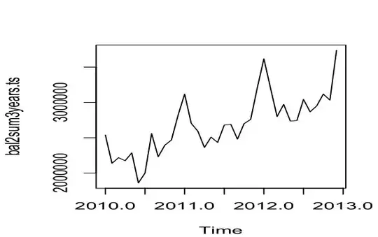
My data is the following time series ( over 3 years, with clear trend upwards and visible seasonality, which seems to be not supported by autocorrelation at lags 12, 24, 36??).
    > bal2sum3years.ts
             Jan     Feb     Mar     Apr     May     Jun     Jul     Aug
    2010 2540346 2139440 2218652 2176167 2287778 1861061 2000102 2560729
    2011 3119573 2704986 2594432 2362869 2509506 2434504 2680088 2689888
    2012 3619060 3204588 2800260 2973428 2737696 2744716 3043868 2867416
             Sep     Oct     Nov     Dec
    2010 2232261 2394644 2468479 2816287
    2011 2480940 2699780 2760268 3206372
    2012 2951516 3119176 3032960 3738256
The model that was suggested by auto.arima(bal2sum3years.ts) gave me the following model:
    Series: bal2sum3years.ts
    ARIMA(0,0,0)(0,1,0)[12] with drift

    Coefficients:
              drift
          31725.567
    s.e.   2651.693

    sigma^2 estimated as 2.43e+10:  log likelihood=-321.02
    AIC=646.04   AICc=646.61   BIC=648.39
However, the acf(bal2sum3years.ts,max.lag=35) does not show acf coefficients higher than 0.3. The seasonality of the data is, however, pretty obvious - spike at the beginning of every year. This is what the series looks like on the graph:
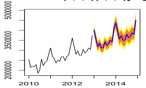
The forecast using fit=Arima(bal2sum3years.ts,seasonal=list(order=c(0,1,0),period=12),include.drift=TRUE) , called by function forecast(fit), results in the next 12months's means being equal to the last 12 months of the data plus constant. This can be seen by calling plot(forecast(fit)),
I have also checked the residuals, which are not autocorrelated but have positive mean ( non zero).
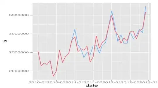
The fit does not model the original time series precisely, in my opinion ( blue the original time series, red is the fitted(fit):
The guestion is, is the model incorrect? Am I missing something? How can I improve the model? It seems that the model literally takes the last 12 months and adds a constant to achieve the next 12 months.
I am a relative beginner in time series forecasting models and statistics.
