Kernel Density Estimate for Cauchy

Question

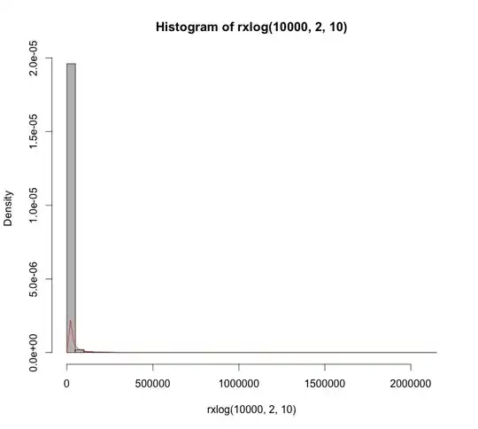
As far as I understand, kernel density estimation does not make any assumptions on the moments of the underlying density, and just requires smoothness. The Cauchy density function is quite smooth. Even still, when I try to do KDE using density() in R for random draws from Cauchy distribution, I get incredibly inaccurate answers:

set.seed(1)
foo <- seq(-50, 50, length = 1e3)
plot(foo, dt(foo, df = 1), type = 'l')
lines(density(rt(1e3, df = 1)), col = "red")

produces this plot:

Repeat the above with different seeds or increasing the sample size can give further erratic estimates. The default kernel is Gaussian in R. Changing the kernel to any of the other options doesn't improve the output.

Question: What assumptions does Cauchy violate for KDEs? If it doesn't, then why do we see KDEs failing so miserably here?

---

Edit: @cdalitz has identified that the problem is where the kde is evaluating the density. The default is 3*bw*range(x), which for Cauchy can be quite large. Which means, by default density tries to estimate the KDE at 512 points sparsely distributed on the x-axis.

To test this, I change the from and to in the density estimation and see that if I run density twice with two sets of evaluating points, so the densities match:

set.seed(1)
samp <- rt(1e4, df = 1)

bd <- 10
den1 <- density(samp, from=-bd, to=bd, n=512)
den2 <- density(samp, from =-2*bd, to = 2*bd,  n =512)

foo <- seq(-50, 50, length = 1e3)
plot(foo, dt(foo, df = 1), type = 'l')
lines(den2, col = "blue", type = "b")
lines(den1, col = "red", type = "b")

This produces the estimates below:

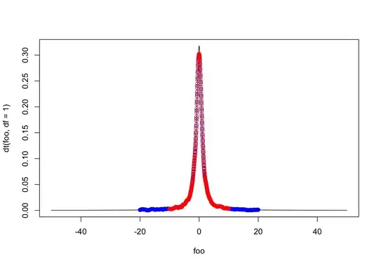
The quality here is much better than before. However, now if instead of 2*bd, I change this to 50*bd, I get that the density estimate even around 0 is very different!

set.seed(1)
samp <- rt(1e4, df = 1)

bd <- 10
den1 <- density(samp, from=-bd, to=bd, n=512)
den2 <- density(samp, from =-50*bd, to = 50*bd,  n =512)

foo <- seq(-50, 50, length = 1e3)
plot(foo, dt(foo, df = 1), type = 'l', ylim = c(0,.7))
lines(den2, col = "blue", type = "b")
lines(den1, col = "red", type = "b")

How does evaluating the density at sparse points change the density evaluation process around $x = 0$ (the bandwidth chosen is the same for both den1 and den2)? The KD estimate at any point $x$ is $$ \hat{f}(x) = \dfrac{1}{nh} \sum_{t=1}^{n} K\left( \dfrac{x - x_i}{h}\right)\,. $$

The density estimate shouldn't change at a given value of $x = a_1$ if the density is also being evaluated at other points. What am I missing here?

Answer 1

The problem lies in the sampling of the x-range by density. By default, density samples 512 values in the range of the data. As the Cauchy distribution has a heavy tail, you will only achieve a very sparse sampling of the density function with the default settings.

If we sample 512 values between -20 and +20, the density approximation is decent, even with the default bandwidth selection rule:

set.seed(1)
foo <- seq(-50, 50, length = 1e3)
plot(foo, dt(foo, df = 1), type = 'l')
lines(density(rt(1e3, df = 1), from=-20, to=20, n=512), col = "red")

Note also that from, to and n only affect the sample points at which the kernel density estimator is evaluated and have no effect on the bandwidth:

> set.seed(1)
> x <- rt(1e3, df = 1)
> density(x, from=-20, to=20, n=512)$bw
[1] 0.351773
> density(x)$bw
[1] 0.351773

Answer 2

In R, the procedure density gives a kernel density estimator (KDE) of data.

In order to get a suitable histogram of the very heavy tailed Cauchy distribution, it is usually necessary to disregard more than a few values in the tails of the sample.

Then in order show the actual Cauchy density curve (black below), it is necessary to adjust the density by dividing by the proportion of the sample plotted in the histogram.

Also, to get a the best KDE (dotted red) you may need to use parameter adj tp adjust the default bandwidth. (I used the default.) Of course, the histogram would be 'smoother' if it had fewer bins; the KDE is made entirely without reference to the histogram.

By adjusting the proportion of the sample plotted, the bandwidth of the KDE, and the sample size, you may be able to improve on my plot below. But the agreement of the density function and the KDE in the the plot below is roughly typical for samples of size 500 to 1000.

R code for figure:

k = diff(pt(c(-4,4),1))
set.seed(2022)
w = rt(1000, 1)        # whole sample, size 1000
y = w[x > -4 & w < 4]  # 861 plotted points
length(y)
[1] 861

hist(y, prob=T, ylim=c(0,.4), br=50, col="skyblue2")
 curve(dt(x,1)/k, add=T, lwd=2)
 lines(density(y), col="red", lwd=2, lty="dotted")

Note: For moderately large samples, the empirical CDF (ECDF) of the sample matches the density function of the population very well. The test statistic $D$ of the Kolmogorov-Smirnov goodness-of-fit test, is the maximum vertical distance between the two.

plot(ecdf(w), lwd=3, col="red", lty="dotted")
 curve(pt(x,1), add=T)
  abline(v=0, col="green2")
  abline(h=0:1, col="green2")

ks.test(w, pt, 1)

        One-sample Kolmogorov-Smirnov test

data:  w
D = 0.018508, p-value = 0.8832
alternative hypothesis: two-sided