What to do when model fails Ljung-Box test?

Question

I have been learning time-series forecasting recently and I am trying to understand the procedure. I would like to find the best model for a daily time series, so far I tried exponential smoothing with ets and also ARIMA with auto.arima, but when I pass both models to Ljung-Box test, they both fail. I would like to know how I could improve the forecast here since I am relatively new and have many questions as I would like to learn more and dive deeper into this field. For example I am familiar with improving the forecast of linear models with AR models where we apply an ARIMA model on the residuals and improve it. But about ets and ARIMA models I am not sure.
Here are the results:

# The forecast for 14 days ahead

auto.arima(ts_d) %>%
  forecast(h = 14) %>%
  autoplot()

and also the result of Ljung-Box test:

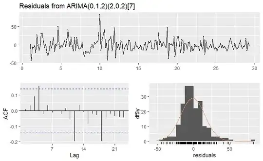
checkresiduals(auto.arima(ts_d))

    Ljung-Box test

data:  Residuals from ARIMA(0,1,2)(2,0,2)[7]
Q* = 16.683, df = 8, p-value = 0.03358

Model df: 6.   Total lags used: 14

The result of exponential smoothing model:

ets(ts_d) %>%
  forecast() %>%
  plot()

And also the result of Ljung-Box test for exponential smoothing:

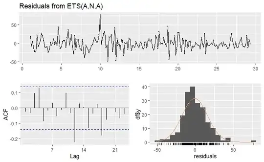
checkresiduals(ets(ts_d))

    Ljung-Box test

data:  Residuals from ETS(A,N,A)
Q* = 21.076, df = 5, p-value = 0.0007837

Model df: 9.   Total lags used: 14

One more thing I don't understand is why I got an error message as follows when I apply a log transformation on my ARIMA model:

Error in auto.arima(ts_d, lambda = 0) : No suitable ARIMA model found In addition: Warning message: The chosen seasonal unit root test encountered an error when testing for the first difference. From stl(): NA/NaN/Inf in foreign function call (arg 1) 0 seasonal differences will be used. Consider using a different unit root test.

Here I also add a reproducible version of my ts:

structure(c(70, 4, 27, 25, 27, 6, 58, 44, 6, 29, 60, 65, 36, 
36, 43, 0, 0, 22, 48, 19, 38, 58, 0, 20, 28, 90, 30, 28, 42, 
9, 26, 42, 48, 42, 76, 49, 15, 49, 33, 32, 54, 34, 62, 22, 27, 
24, 33, 47, 18, 13, 2, 10, 8, 13, 12, 20, 29, 7, 28, 26, 33, 
36, 51, 114, 9, 42, 57, 75, 30, 41, 15, 28, 49, 62, 30, 37, 85, 
9, 31, 32, 45, 27, 45, 59, 7, 19, 32, 44, 21, 49, 61, 12, 10, 
24, 28, 36, 36, 43, 12, 15, 27, 21, 15, 35, 48, 6, 15, 36, 36, 
36, 24, 28, 6, 30, 43, 18, 60, 32, 43, 14, 33, 37, 27, 30, 79, 
3, 22, 29, 36, 26, 56, 13, 16, 44, 53, 34, 8, 53, 44, 4, 32, 
38, 22, 29, 49, 18, 15, 14, 21, 29, 20, 36, 23, 3, 33, 24, 16, 
45, 11, 34, 9, 14, 21, 23, 21, 39, 22, 3, 13, 6, 15, 18, 31, 
15, 9, 9, 12, 9, 3, 15, 27, 30, 24, 12, 3, 18, 15, 9, 9, 21, 
27, 9, 6, 12, 12, 30, 3, 24, 9), .Tsp = c(1, 29.2857142857143, 
7), class = "ts")

Thank you very much in advance for your time and please forgive me if my question seems so basic as I am quite naive in the field but very eager to improve.

Answer 1

Regarding exponential smoothing yielding autocorrelated residuals, it depends on how strong the autocorrelation is (magnitude, not only statistical significance). If it is strong, consider using another model or modelling the residuals and adjusting your forecasts accordingly.

Thank you very much dear Mr. Hardy. I managed to fix this by playing with $p$, $d$ and $q$ parameters. I would like to ask would it be weird if I could use a model like Arima(ts_d2, order = c(20, 2, 2), lambda = 0.3) for example with a $p$ of 20 so that all residuals become independent with $p$-value also greater than 0.05?

There is the bias-variance trade-off. If you have a complex model like yours, its bias may be low but variance will be high, unless you time series is very long. That will have a negative impact on forecast accuracy. Consider using regularized estimation or setting some coefficients to zero to mitigate that. Consider using auto.arima for model selection, as that model selection algorithm is tuned specifically with forecast accuracy in mind.

I used auto.arima to get an ARIMA(0,1,1) and my $p$-value is now 0.4505 and AICc is around 61.05 with only one lag outside the blue dotted lines in ACF diagram. <...> Based on what you mentioned above so with this new $p$-value if we have only one or two lags outside the blue dotted lines, does it mean that our model fitted the data quite well? which one actually defines the situation better?

The new model with its diagnostics sounds quite good to me. If the lags that stick out are distant lags (not the first few) and/or they stick out only a little bit, then they are probably harmless. Note that under the null hypothesis of no autocorrelation, on average 1 out of 20 lags would stick out of the confidence bounds by pure chance.

Is it really essential to partition the data to train and test for ARIMA models? Because in this case I didn't do that.

In a time series setting, this is quite costly, as you generally cannot do leave-one-out or $k$-fold cross validation like you could in a cross section. But for a fair evaluation of predictive performance, splitting the data into training and test subsamples is hard to beat. If you were not doing any model selection, AIC would be a fair estimate of the model's expected loss on new data in terms of twice the negative log-likelihood. But when doing model selection, the selected model suffers from the winner's curse, so the AIC of the winner is overly optimistic. Thus better consider using a test subset to evaluate your model.