5

I'm struggling with a proof of the normal equation, so I posted a question which hopefully will get resolved soon. However, I mentioned there that I'm uncomfortable with the proofs dealing with matrix calculus, particularly when it comes to derivatives of product of vectors or product of matrices and vectors. Furthermore, there are a couple of "layout conventions" which are not even used consistently. Because of this, I thought I could get rid of all that insanity by using tensor notation instead.

In relation to the normal equation question, I would be very interested in looking at a proof of this equation (here you can see the context):

$$\beta = (X^{T}X)^{-1}X^{T}{\bf{y}}$$

using tensor notation.

And as a more general request, I'd like to get an advice on the issue of dealing with matrix calculus and derivatives. Particularly, I want to hear about your approach when you have to calculate something of this kind given the inconsistencies in notations and non-intuitive nature of some identities. Do you consult Wikipedia or some handbook every time you want to calculate a derivative of some product of vectors or matrices? Do you memorize some recurrent identities? Do you know an alternative procedure?

kjetil b halvorsen
  • 63,378
  • 26
  • 142
  • 467
Robert Smith
  • 3,191
  • 3
  • 30
  • 46
  • 1
    Offhand I'm familiar with at least a half dozen conventions that could validly be called "tensor notation." One of them is infamously called the ["debauch of indices"](http://books.google.com/books?id=_pNwvEu-dloC&pg=PA69&dq=debauch+of+indices+Cartan+geometrie+des+espaces+de+riemann&hl=en&sa=X&ei=mFdaUYX_K7LA4APO34DwAw&ved=0CDEQ6AEwAA#v=onepage&q=debauch%20of%20indices%20Cartan%20geometrie%20des%20espaces%20de%20riemann&f=false): I hope that's not the one you mean! But what exactly do you want? – whuber Apr 02 '13 at 04:01
  • I didn't know there are so many conventions. I had in mind something like this: https://docs.google.com/viewer?url=http%3A%2F%2Fwww.atmos.washington.edu%2F~dennis%2FMatrixCalculus.pdf in page 4. – Robert Smith Apr 02 '13 at 04:04
  • 1
    That document uses at least two notations. Notice how quickly the author abandons the multiple-subscript notation for the simpler and clearer vector-matrix notation. Following that procedure yourself is already pretty good advice--if you get tied up tracking subscripts, you will lose sight of what's really going on. – whuber Apr 02 '13 at 04:22
  • That is actually true. I don't know what you mean by "the author abandons the multiple-subscript notation for the simpler and clearer vector-matrix notation", though. Which part are you referring to? – Robert Smith Apr 02 '13 at 04:38
  • At the beginning, equation (1)--a partially written-out array--, equation (2)--the "$[a_{ij}]$" notation--, and the symbol "$A$" at the end of the subsequent paragraph all refer to the same mathematical object. That's three notations right there. Throughout the rest of the document, the first notation is used rarely (eqs (24) and (67) only) and occasionally in abbreviated (block-matrix) form, as in equation (19); the second notation is almost as rarely used (as in equation (13)); and the third notation--which has no subscripts--is used hundreds of times. – whuber Apr 02 '13 at 12:34
  • I think the second notation is used to prove the non-intuitive identities of matrix calculus (using the notation without indexes) – Robert Smith Apr 02 '13 at 16:15
  • @RobertSmith in your link page4, I see a Jacobian but no 'tensor' – caub May 04 '14 at 09:41
  • @cc Starts in page 4. The propositions that follow are good examples. – Robert Smith May 04 '14 at 15:22
  • @RobertSmith I see the term "partitioned matrices" (still not "tensor") but I guess it's similar – caub May 04 '14 at 15:49
  • @cc A matrix is a especial case of a second order tensor. Maybe you're confusing tensors with the idea of tensor notation (using indexes, operations of contraction, etc) – Robert Smith May 04 '14 at 16:39

2 Answers2

7

A "modern" (post-1900) view of tensors is a geometric one. Perhaps the clearest notation would therefore be a figure, because the "normal equations" are nothing more than a familiar, ages-old theorem of plane geometry!

As a point of departure, let's begin with an expression from your previous question. The setting is Ordinary least squares (OLS). The data are the "design matrix" $(x_{i,j})$, $1 \le i \le n$, $1 \le j \le p$ of "independent variables" and a vector of values of the "dependent variable" $y = (y_i)$, $1 \le i \le n$; each dependent value $y_i$ is associated with the $p$-tuple of independent values $(x_{i,1}, x_{i,2}, \ldots, x_{i,p}).$

OLS aims to find a vector $\beta = (\beta_1, \beta_2, \ldots, \beta_p)$ minimizing the sum of squares of residuals

$$\sum_{i=1}^n\left(y_i - \sum_{j=1}^p \left(x_{i,j}\beta_j\right)\right)^2.$$

Geometrically, the inner sum of products represents the application of the linear transformation determined by the matrix $x = (x_{i,j})$ to the $p$-vector $\beta$. As such we conceive of $x$ as representing a map $x: \mathbb{R}^p\to \mathbb{R}^n$. The outer sum is the usual Pythagorean formula for the Euclidean distance. Geometrically, then,

OLS seeks a vector $\hat\beta \in \mathbb{R}^p$ for which $x\hat\beta\in \mathbb{R}^n$ is as close to $y$ as possible.

The test of this is to take any other vector $\beta'\in \mathbb{R}^p$ and to compare distances within the triangle formed by the three points $y$, $x\hat\beta$, and $x\beta'$:

Figure

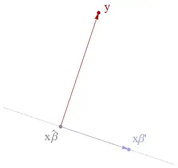
According to Euclid, three (distinct) points determine a plane, so the figure is utterly faithful: all our work is done within this plane.

We also know from Euclid that the ray $y - x\hat\beta$ must be perpendicular to the ray $x\beta' - x\hat\beta$. (This is the heart of the matter; in making this observation, we are really done and all that remains is to write down an equation expressing this perpendicularity.) Modern geometry has several notations for perpendicularity, which involves the (usual) "dot product" or positive-definite linear form (a "tensor of type $(2,0)$" if you wish). I will write it as $\langle\ ,\ \rangle$, whence we have deduced

$$\langle x\beta', y-x\hat\beta\rangle = 0$$

for all $\beta\in\mathbb{R}^p$. Because the usual dot product of two vectors in $\mathbb{R}^n$ is

$$\langle u, v\rangle = u^\intercal v,$$

the preceding may be written

$$\beta'^\intercal x^\intercal (y - x\hat\beta) = 0.$$

Geometrically, this says that the linear transformation from $\mathbb{R}^{p*}\to\mathbb{R}^n$ defined by applying $x^\intercal (y - x\hat\beta)$ to $\beta'^\intercal$ is the zero transformation, whence its matrix representation must be identically zero:

$$x^\intercal (y - x\hat\beta) = 0.$$

We are done; the conventional notation

$$\hat\beta = \left(x^\intercal x\right)^{-}\left(x^\intercal y\right)$$

(where "$\left(\right)^{-}$" represents a generalized inverse) is merely an algebraically suggestive way of stating the same thing. Most computations do not actually compute the (generalized) inverse but instead solve the preceding equation directly.


If, as an educational exercise, you really, really want to write things out in coordinates, then I would recommend adopting coordinates appropriate to this configuration. Choosing an orthonormal basis for $\mathbb{R}^n$ adapted to the plane determined by $y$ and $x\beta'$ for some arbitrary $\beta'$ allows you to forget the remaining $n-2$ coordinates, because they will be constantly $0$. Whence $y$ can be written $(\eta_1, \eta_2)$, $x$ can be written $(\xi_1, \xi_2)$, and $\beta'$ can be considered a number. We seek to minimize

$$\sum_{i=1}^n\left(y_i - \sum_{j=1}^p \left(x_{i,j}\beta_j\right)\right)^2=\left(\eta_1 - \xi_1 \beta\right)^2 + \left(\eta_2 - \xi_2 \beta\right)^2.$$

OLS claims that this is achieved for

$$\hat\beta = \left(x^\intercal x\right)^{-}\left(x^\intercal y\right)=\left(\xi_1^2 + \xi_2^2\right)^{-1}\left(\xi_1 \eta_1 + \xi_2 \eta_2\right)$$

provided $\xi_1^2 + \xi_2^2 \ne 0$. An elementary way to show this is to expand the former expression into powers of $\beta$ and apply the Quadratic Formula.

whuber
  • 281,159
  • 54
  • 637
  • 1,101
  • 1
    Thanks! I was aware of the geometric proof but I'm more interested in a proof actively using tensors in order to get the terms of $\beta$ – Robert Smith Apr 02 '13 at 16:18
  • 1
    This proof *does* use tensors! – whuber Apr 02 '13 at 17:28
  • Yes, but the tensors are not central to the proof. Basically, I want to look at the proof because I'd like to get a taste of how to deal with the derivative to minimize the error function in tensor notation. – Robert Smith Apr 02 '13 at 17:41
  • That might be a question for the math site rather than here. – whuber Apr 02 '13 at 17:43
  • 1
    It could be but I have found that here I get more relevant answers on these topics than in math.stackexchange – Robert Smith Apr 02 '13 at 17:53
  • Questions that are purely about mathematical techniques, such as how to take derivatives or manipulate indices, are not on topic here. The trick is to edit your question to keep it focused on matters of statistical interest, but if that cannot be done, we will migrate the question for you. – whuber Apr 02 '13 at 17:55
  • I think it's pretty relevant here since the question deals with linear regression and the request for advice is much more relevant here than in math.stackexchange (you know, mathematicians are comfortable with tensors but in a more abstract setting so they don't have to struggle with this kind of calculation.) – Robert Smith Apr 02 '13 at 19:13
2

The proof for the normal equation (in matrix notation):

Let $J$ be the cost function for the linear regression given by

$$ \begin{aligned} J &= \vert\vert {\bf X}{\bf w} - {\bf t}\vert\vert^2\\ &= \left({\bf X}{\bf w} - {\bf t}\right)^T\left({\bf X}{\bf w} - {\bf t}\right)\\ &= \left({\bf w}^T{\bf X}^T - {\bf t}^T\right)\left({\bf X}{\bf w} - {\bf t}\right)\\ &= {\bf w}^T{\bf X}^T{\bf X}{\bf w} - 2{\bf w}^T{\bf X}^T{\bf t}-{\bf t}^T{\bf t}\\ &= \text{Tr}\left({\bf w}{\bf w}^T{\bf X}^T{\bf X}\right)- 2{\bf w}^T{\bf X}^T{\bf t}-{\bf t}^T{\bf t}\\ \end{aligned} $$

Noting that $\frac{\partial \text{Tr}(AB)}{A} = B^T$, and $\frac{\partial}{\partial {\bf x}}{\bf x}^T{\bf a} ={\bf a}$. We get

$$ \begin{aligned} \frac{\partial J}{\partial {\bf w}} &= \frac{\partial}{\partial {\bf w}}\left( \text{Tr}\left({\bf w}{\bf w}^T{\bf X}^T{\bf X}\right)- 2{\bf w}^T{\bf X}^T{\bf t}-{\bf t}^T{\bf t}\right)\\ &= ({\bf X}^T{\bf X})\frac{\partial {\bf w}{\bf w}^T}{{\bf w}} - 2{\bf X}^T{\bf t}\\ &= ({\bf X}^T{\bf X})2{\bf w} - 2{\bf X}^T{\bf t}\\ \end{aligned} $$

Setting this last value to $\bf 0$ and solving for ${\bf w}$ we get:

$$ {\bf w} =({\bf X}^T{\bf X})^{-1}{\bf X}^T{\bf t} $$


As we can see from the proof above, there exists a consistent layout conventions in dealing with matrix calculus, the same way that there exist a layout convention in calculus under the real line. The key to understand matrix derivatives, as with derivatives for functions $f:\mathbb{R}\to\mathbb{R}$ is practice. Take a look at the Matrix Cookbook for further reference.