Since the beta distribution has only two parameters, but you want to satisfy three conditions, you will probably not be able to get a perfect fit.
One possibility would be to define an objective function that takes two parameters $(\alpha,\beta)$ and calculates the deviation between the quantiles and the mode of the corresponding beta distribution on the one hand, and your target values on the other hand. Then run a straightforward optimizer over it. If you use the sum of the squared deviations, this is easy to numerically optimize.
foo <- optim(par=c(1.2,1.2),
    fn=function(par)(qbeta(0.25,par[1],par[2])-0.3)^2+ # first quartile
                    (qbeta(0.75,par[1],par[2])-0.9)^2+ # third quartile
                    ((par[1]-1)/(sum(par)-2)-0.6)^2,   # mode
    method="L-BFGS-B",lower=1)
Unfortunately, it turns out that the result fits your conditions on the first quartile and the mode rather well - but the third quartile quite badly. Essentially, making the beta distribution conform to the first two conditions makes it very hard to also satisfy the third one.
> qbeta(c(0.25,0.75),foo$par[1],foo$par[2])
[1] 0.2964684 0.7504854
> (foo$par[1]-1)/(sum(foo$par)-2)
[1] 0.6273578
Here is the density:
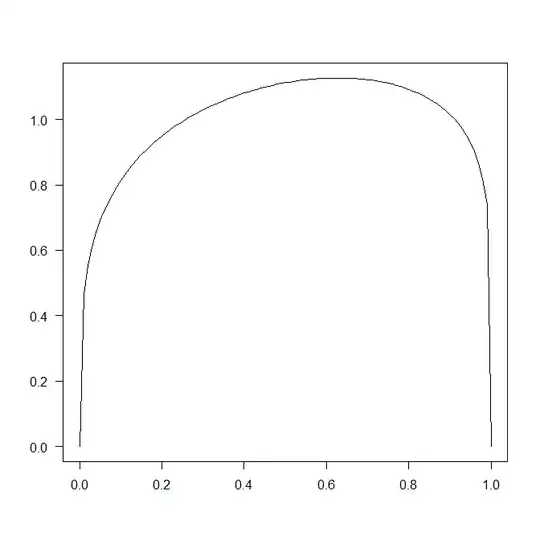
xx <- seq(0,1,by=0.01)
plot(xx,dbeta(xx,foo$par[1],foo$par[2]),type="l",las=1,xlab="",ylab="")
You could start playing around with weights on your three conditions, but then of course, as you improve the third quartile, the other two conditions suffer. Or you could try looking for a three-parameter generalization of the beta, which you might be able to match exactly to your requirements.
