Model Verification for Gamma GLMM, different between qqplot and DHARMA

Question

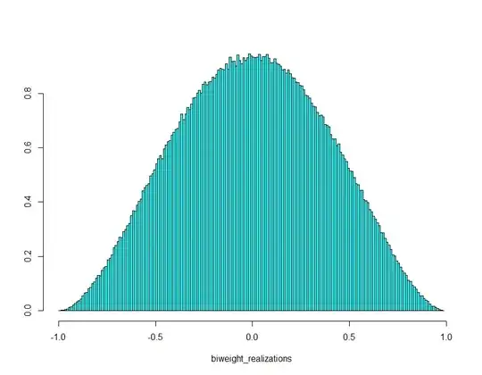
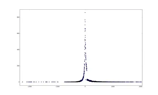
I am working with a dataset where the response variable looks like an in-between of normal and gamma distribution

Edit: Including model formula and output, as requested, below



I’m using lme4 because I also have a random effect structure (treatment|farm_id) In calculating AICc values of the null models for both distributions I got - gamma AICc (-158.3) and normal AICc (-61.5)

Implying the gamma is a better fit, correct?

During model verification I’ve run into some issues though. I’ve mainly been following the advice from this post: What are the assumptions of a Gamma GLM or GLMM for hypothesis testing?

GAMMA MODEL VERIFICATION

res.gammaModel <- resid(gammaModel)
qqnorm(res.gammaModel)
qqline(res.gammaModel)›



ypred = predict(gammaModel)
res = residuals(gammaModel, type = 'pearson')
plot(ypred,res)



I feel like the QQplot isn’t great but isn’t bad and the residuals versus predicted aren’t showing patterns

plot(y = res, x = scaled.originalData$treatment)



plot(y = res, x = scaled.originalData$explanatoryVariable)



But then…

plot(y = res.gammaModel, x = originalData$responseVariable)



Here I can’t use x = gammaModel$Obs because its a glmm I guess? And I have some NA values in my data that I needed to get rid of so maybe thats where I went wrong?

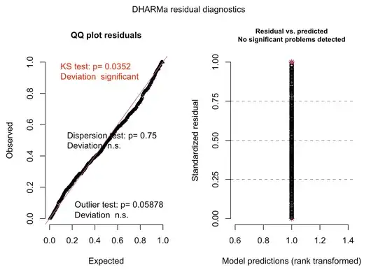
Furthermore using DHARMA for the gamma distribution



I’m not really sure where I’m going wrong? I’m using model.sel() and these plots are from the top model (delta AICc only 1 better than the null model).

On the otherhand, the top model of the model.sel() for the normal distribution set of models was the null model (by delta AICc 4) and the DHARMA QQ plot looked better

 Any advice would be greatly appreciated!

Edit- Formulas and output - on another note, I realized I am using REML for lmer and ML for glmer - I include the output for an lmer run on ML at the end...

gammalmm <- glmer(response  ~ exVar + (treatment|farm_id), data=scaled.originalData, family = Gamma, control=glmerControl(optimizer="bobyqa", optCtrl=list(maxfun=100000)))

    Generalized linear mixed model fit by maximum likelihood (Laplace
  Approximation) [glmerMod]
 Family: Gamma  ( inverse )
Formula: response ~ exVar + (treatment | farm_id)
   Data: scaled.originalData
      AIC       BIC    logLik  deviance  df.resid 
-160.2394 -120.6222   89.1197 -178.2394       594 
Random effects:
 Groups      Name        Std.Dev. Corr       
 farm_id     (Intercept) 0.3859              
             treatmentBG 0.2714   -0.91      
             treatmentCC 0.3824    0.12 -0.17
 Residual                0.3192              
Number of obs: 603, groups:  farm_id, 9
Fixed Effects:
 (Intercept)         exVar  
     1.20526       0.01206 


lmm <- lmer(response  ~ 1 + (treatment|farm_id), data=scaled.originalData)

Linear mixed model fit by REML ['lmerMod']
Formula: response ~ 1 + (treatment | farm_id)
   Data: scaled.originalData
REML criterion at convergence: -77.7584
Random effects:
 Groups      Name        Std.Dev. Corr       
 farm_id     (Intercept) 0.25875             
             treatmentBG 0.09519  -0.47      
             treatmentCC 0.18723   0.00 -0.31
 Residual                0.21336             
Number of obs: 603, groups:  farm_id, 9
Fixed Effects:
(Intercept)  
     0.7496 


Linear mixed model fit by maximum likelihood  ['lmerMod']
Formula: response ~ 1 + (treatment | farm_id)
   Data: scaled.originalData
     AIC      BIC   logLik deviance df.resid 
-65.0964 -29.8811  40.5482 -81.0964      595 
Random effects:
 Groups      Name        Std.Dev. Corr       
 vfarm_id    (Intercept) 0.24687             
             treatmentBG 0.09501  -0.49      
             treatmentCC 0.18716   0.00 -0.31
 Residual                0.21337             
Number of obs: 603, groups:  farm_id, 9
Fixed Effects:
(Intercept)  
     0.7495  

And the DHARMA for the lmm fit with Maximum likelihood