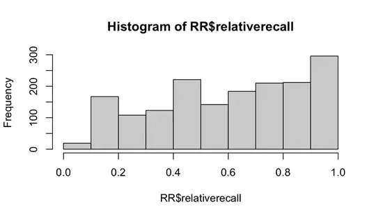
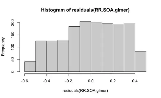
As commented by @Dave and as probably pointed out many times on CV (e.g. here and here), you shouldn't worry about the marginal ("overall") distribution of the response, but the conditional distribution (which you have, by looking at the histogram of the residuals).
Depending on what you're doing, you might not even need to worry about the non-Normality in the residuals/conditional distribution. Linear models (including LMM) are pretty robust to moderate amounts of non-Normality. That said, if you are modeling responses on a 0-1 scale, you might want to worry about issues like nonlinearity, ceiling effects (i.e. what happens when relative recall gets close to a boundary at 1?), and heteroscedasticity, all of which are potentially bigger issues than the mere lack of Normality in the residuals.
If relative recall is measured on a continuous (0,1) scale, and if there are no exact 0/1 values, it probably makes most sense to model it as a Beta distribution. (Also assuming that this is not a ratio with a known denominator, e.g. 5/17, in which case it's probably best to use a binomial model). There are several R packages that can fit mixed-effect beta models (glmmTMB, brms, mgcv, INLA, gamlss).
For example, if the number of items offered to each subject in each category (i.e. the number of items making up the denominator of each computed relativerecall observation) is stored as N in the data set, then the model fit
model <- FUN(relativerecall ~ A*B + (1|subject),
           data = df,
           weights = N,
           family=binomial)
where FUN is either lme4::glmer or glmmTMB::glmmTMB, should work and should give nearly identical results. The weights argument is important ...
If you have a significant number of exact-0 or exact-1 values (so many that "squeezing" slightly to get them off the boundary seems dicey) you'll need a zero-inflated or zero-one-inflated Beta mixed model, which limits your choices slightly further.

