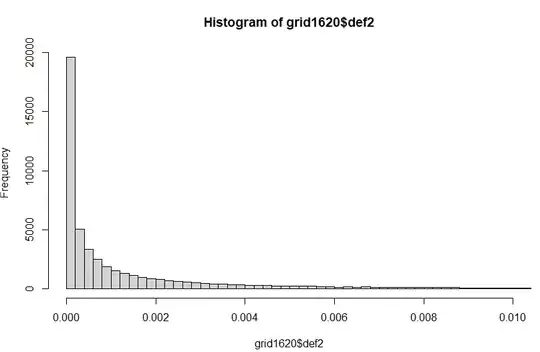
I'm running a regression in R-INLA, where the response variable is proportion of grid squares suffering deforestation (by year, over a 20-year period). Setting the response for the last 5 years to NA and re-running the model fit (which is the recommended way to do predictions in INLA), I get a good Spearman's rank correlation between observed and predicted values, so the model does well at predicting relative risk, but the actual and predicted values look very different and the RMSE is high. The actual values are overdispersed and a lot of grid squares have zero deforestation:
...compare this to the predictions for these 5 years from model$summary.fitted.values$mean
Can I set priors to improve the prediction? How would you do this with an INLA beta distribution? (INLA uses mean and precision, not alpha and beta)
Here is the model ('f' is a spatial random effect, I did try adding 'year' as a variable too but it had no effect)
formula <- deforestation ~ cost + elevation + landcover +
  f(gridID, model = "bym", graph = lattice.adj, scale.model=TRUE)
model <- inla(formula, data = gridPolygons, family = "beta",
                  control.family=list(link='logit'),
                  control.predictor=list(link=1, compute=TRUE),
                  control.compute=list(dic=TRUE, cpo=TRUE, waic=TRUE))
To set priors I think the code would be something like this, added to the INLA call:
          control.fixed=list(mean=0.001, prec=50,
                             mean.intercept=0, prec.intercept=0.001))
P.S. the area of my grid squares varies, which is why I used a proportion rather than e.g. count of 'deforested' pixels with a negative binomial distribution.

