0

I am ripping my head off right now. I have beensitting all day, and tried to solve this assigment i have in statistics.

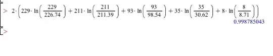
I have 5 observations: 229, 211, 93, 35, 8
I have 5 Expected observations: 226.74, 211.39, 98.54, 30.62, 8.71

I have to make a goodness of fit test of these numbers therefore i started to find G:

2 * (229 * ln(229 / (226.74)) + 211 * ln(211 / (211.39)) + 93 * 
           ln(93 / (98.54)) + 35 * ln(35 / (30.62)) + 
           8 * ln(8 / (8.71))) = 0.9987

or

enter image description here

So now i have my:

lower value = 0.9987 and
df = 4

So now i have to find my pvalue through cdc(lower value, df) ? I cant seem to get anything right here, and i dont know if i have done it the correct way until now? Do anyone have an idea on how i could solve this? And incase how i type it in R or Maple?

Carl
  • 11,532
  • 7
  • 45
  • 102
  • What is the distribution of your observations? – Ferdinand.kraft Mar 26 '13 at 18:02
  • Thank so much for your answers. Im just at work right now, but Im Gonna look when i Come home. There was a student who made te assigement, and he Said the correct result was 0.81. But i cannot figure out if that is true? A little bit stupid question. What is the distribution? Best Regards Mads –  Mar 27 '13 at 19:41
  • 1
    @user23599 That student might have used three degrees of freedom instead of four. It's not possible to determine from your question whether that is correct or not. BTW, a good way to avoid questions you fear might be stupid is to [do a quick search first](https://www.google.com/search?q=distribution+definition+statistics). – whuber Mar 27 '13 at 19:51

2 Answers2

2

You are doing a G-test, upon which Chi-squared tests are based.

Firstly, (as @whuber and @ferdinand-kraft have mentioned) the number of degrees of freedom should be checked given your expected values are not uniform, but assuming it's 4 and if using R, then to get your P-value, you need to do:

obs <- c(229,211,93,35,8)
exp <- c(226.74,211.39,98.54,30.62,8.71)
(q <- 2*sum(obs*log(obs/exp)))

which gives: 0.9987848

then for the P-value:

(p <- 1-pchisq(q,4))

which gives: 0.9099802


If you wanted to do a Chi-squared test, then only the q is different:

(q <- sum((obs-exp)^2/exp))

which gives: 1.019117 and a corresponding P-value of: 0.9068835

sqrt
  • 450
  • 2
  • 13
  • The code looks good and making the connection with chi-squared is even better. But how have you determined that the degrees of freedom must be $4$? I can find no information in the question that tells us anything about that (although I see the O.P. has made the same assumption, but again with no apparent justification). – whuber Mar 27 '13 at 14:13
  • Very good point! the questioner should give more info on how the expected values were calculated. For one dimensional data, the number of degrees of freedom is _n-1_, hence _4_ in this case. This can be different if the observations don't come from a uniform distribution. Given the expected values here, they do not come from a uniform, so the number of degrees of freedom may be different. More details for this at [wikipedia](http://en.wikipedia.org/wiki/Pearson%27s_chi-squared_test#Other_distributions) – sqrt Mar 27 '13 at 15:15
  • 1
    Your statement about "one dimensional data" is only sometimes correct and often is wrong. What is true is that the degrees of freedom *usually* are equal to the data count minus the number of parameters used to compute the expected values. For instance, if the five observations in the question are bin counts and the five expected values are based on fitting (say) a three-parameter lognormal distribution using maximum likelihood, then there are only two degrees of freedom. For more about this, please visit [How to Understand Degrees of Freedom?](http://stats.stackexchange.com/questions/16921). – whuber Mar 27 '13 at 15:57
  • Thank you so much for the answer. Richard you wrote the resultant with q and the p value. But what do i need to do with those two numbers? Best Regards Mads –  Mar 29 '13 at 21:28
  • q is the $\chi^2$ test statistic. p can be interpreted as the probability of observing results as extreme as yours, given that the null hypothesis is true. The lower the p, then the less likely the null hypothesis explains the results. Here, the null hypothesis is that your observed values are drawn from a particular distribution, i.e. your expected values. – sqrt Mar 30 '13 at 10:27
0

In R the natural logarithm function is "log", so a global replace produces:

> 2 * (229 * log(229 / (226.74)) + 211 * log(211 / (211.39)) + 93 * 
+            log(93 / (98.54)) + 35 * log(35 / (30.62)) + 
+            8 * log(8 / (8.71)))
[1] 0.9987848

You can compare that with what the formula would have produced if there were complete agreement with expected (somewhat trivially since you should have been able to see this by inspection knowing log(1) == 0):

> 2 * (229 * log(229 / 229) + 211 * log(211 / 211) + 93 * 
+            log(93 / 93) + 35 * log(35 / 35) + 
+            8 * log(8 / 8))
[1] 0

You need to know the distribution of that goodness of fit statistic if you are going to make any inferences. A chi-square GOF would be looking at sums of (expected-observed)^2/expected whereas this GOF is on a log-scale, hence the factor of 2 at the beginning. It bears some resemblance to a log-likelihood expression. You should do some further reading in your textbook.

DWin
  • 7,005
  • 17
  • 32