1

Sometimes data extracted from reports do not have individual values, like 4, 23, 43, but grouped together like this:

income level people in this group
10k to 20k 44
20k to 40k 240
40k to 80k 400
80k to 100k 130

What is the best way to describe this situation in statistics, and how to calculate the mean value?

At first, I thought about multiplying the mid value of the first row by the number of people, i.e.:

mean = ((15k x 44) + (30k x 240) + (60k x 400) + (90k * 130))/(44 + 240 + 400 + 130)

However, I feel since the distribution is skewed, the mid point doesn't represent the mean value in each group, and thus the calculation above is wrong.

I also thought about using weighted arithmetic mean, but I am not sure.

What is the statistic tool to deal with this sort of problem?

DifferentialPleiometry
  • 2,274
  • 1
  • 11
  • 27
samOz
  • 11
  • 1
  • Your table is basically a histogram. You could plot it to further verify if the data is skewed. – DifferentialPleiometry Jun 23 '21 at 02:31
  • 2
    To a good first approximation, income distribution will be closer to symmetric on logarithmic scale than on the original scales. So an alternative would be to work with the geometric mean and similarly the geometric means of the interval end-points. You don't spell it out here but it's common that the uppermost income interval is reported as open-ended, which compounds the problem. – Nick Cox Jun 23 '21 at 07:48
  • See our posts on [Sheppard's corrections](https://stats.stackexchange.com/search?tab=votes&q=sheppard%20correction). Although the duplicate is explicitly about estimating the SD, it also shows how to estimate the mean (and any other moment). The question and its answers present at least three standard methods. – whuber Jun 23 '21 at 16:59

2 Answers2

2

Because your data is binned into intervals, you cannot really calculate the original sample mean because you should not make up information that you don't have access to. However, you have a couple of options.

Option 1

Your first option, which is the one many people take, is to calculate the mean based on the midpoints. This approach is an estimation subject to binning error. This is what you've done in your original post.

Option 2

Your second option is my preferred option, which is calculate an interval that the mean sits within. This can be done with the use of interval arithmetic. It has the following rules for $x_1,x_2,y_1,y_2 \in \mathbb{R}$:

$$[x_1, x_2] + [y_1, y_2] = [x_1 + y_1, x_2 + y_2]$$ $$[x_1, x_2] - [y_1, y_2] = [x_1 - y_1, x_2 - y_2]$$ $$[x_1, x_2] \cdot [y_1, y_2] = [\min \{x_1 y_1, x_1y_2,x_2y_1, x_2y_2 \}, \max \{x_1 y_1, x_1y_2,x_2y_1, x_2y_2 \}]$$ $$\frac{[x_1, x_2]}{[y_1, y_2]} = [x_1, x_2] \cdot \frac{1}{[y_1, y_2]}$$ where $$\frac{1}{[y_1, y_2]} = \begin{cases} \left[\frac{1}{y_2}, \frac{1}{y_1}\right] & 0 \not\in [y_1,y_2] \\ \left(-\infty, \frac{1}{y_1}\right] & y_1 \neq 0 \land y_2 = 0 \\ \left[\frac{1}{y_2},\infty\right) & y_1 = 0 \land y_2 \neq 0 \\ \left(-\infty, \frac{1}{y_1}\right] \cup \left[\frac{1}{y_2},\infty\right) & 0 \in (y_1, y_2) \end{cases}$$

Note that for the above rules a constant $\alpha \in \mathbb{R}$ can be thought of as the interval $[\alpha, \alpha]$ for the purposes of combining intervals with scalars.

In your case, the following can be done quickly in the Python interpreter.

Python 3.6.9
>>> import numpy as np
>>> intervals =[[10,20], [20,40], [40, 80], [80,100]]
>>> weights = [44, 240, 400, 130]
>>> result = 0
>>> for i,j in zip(intervals, weights):
...     result += np.array(i) * j
...
>>> result / np.sum(weights)
array([38.86977887, 68.15724816])

Thus the mean income sits somewhere within \$$[38869.78, 68157.25]$.

DifferentialPleiometry
  • 2,274
  • 1
  • 11
  • 27
  • 1
    For additional descriptions of interval arithmetic, [search our site](https://stats.stackexchange.com/search?tab=votes&q=%22interval%20arithmetic%22). – whuber Jun 23 '21 at 17:02
  • Also note that the arithmetic as defined above allows for polynomials, including Taylor series approximations of exponentials, logarithms, trigonometric, and hyperbolic functions among others. – DifferentialPleiometry Jun 23 '21 at 17:25
  • I think it's more complicated than that. You cannot just apply a polynomial function to all the left endpoints and then to all the right endpoints to determine the resultant interval, for instance; nor can you apply a generalization of the product formula you give. (The problem is that local extrema may occur within the interiors of the intervals). For nonlinear functions you basically have to optimize the function subject to the interval constraints. – whuber Jun 23 '21 at 17:28
  • You're right @whuber that it isn't as simple as applying all the left and right endpoints in general. It depends on the properties of the function. See the [wiki page](https://en.wikipedia.org/wiki/Interval_arithmetic) on handling broader classes of functions. – DifferentialPleiometry Jun 23 '21 at 17:38
1

As an approximation, assume all observations within an interval are located at its center.

Then you have four midpoints $m_j$ with corresponding frequencies $f_j$ for $j = 1,2,3,4.$ where $n = \sum_j f_n = 814.$ Then $\bar X \approx \frac 1n\sum_j f_jm_j = 53.51,$ and $S = \sqrt{S^2} = 21.84,$ in thousands of dollars, where $S^2 \approx \frac{1}{n-1}\sum f_j(m_j-\bar X)^2.$ [Using R.]

m = c(15, 30, 60, 90)
f = c(44, 240, 400, 130)
[1] 814
a = sum(f*m)/n;  a
[1] 53.51351
s = sqrt(sum(f*(m-a)^2)/(n-1)); s
[1] 21.84175

A more elaborate and perhaps slightly more accurate method is to 'reconstruct' the sample by assuming that observations are spread uniformly at random in their respective intervals. Notice that this is a random reconstruction and additional runs of the 'reconstruction' program (without using the set.seed statement) will give slightly different answers.

set.seed(623)
x = c(runif(44, 10, 20), runif(240, 20, 40),
      runif(400,40, 80), runif(130, 80,100))
mean(x);  sd(x)
[1] 53.84582
[1] 23.48832

The approximate mean $\bar X \approx 53.8$ and standard deviation $S\approx 23.5$ are not much different from the previous approximations.

A histogram based on the given intervals roughly suggests the shape of the sample from which such a sample might have been taken. It seems unlikely that the distribution of if incomes is normal. [Tick marks. from rug, along the horizontal axis show the locations of the reconstructed data values.]

hist(x, br=c(10,20,40,80,100)); rug(x)

enter image description here

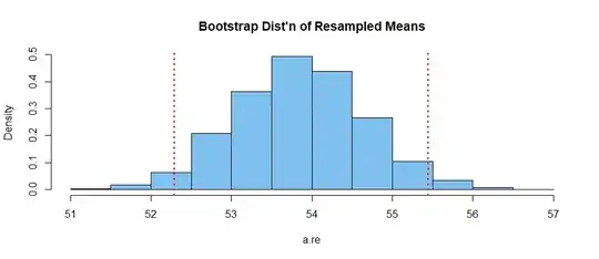
Using the reconstructed the sample, one can get one kind of 95% bootstrap confidence interval $(52.3,\, 55.4)$, in which the population mean $\mu$ might lie.

set.seed(2021)
a.re = replicate( 4000, mean(sample(x,rep=T)) )
ci = quantile(a.re, c(.025,.975)); ci
    2.5%    97.5% 
52.28877 55.44453 

hist(a.re, prob=T)
hdr = "Bootstrap Dist'n of Resampled Means"
hist(a.re, prob=T, col="skyblue2", main=hdr)
 abline(v=ci, col="red", lwd=2, lty="dotted")

enter image description here

Note: As @NickCox has suggested, alternate methods of approximation and reconstruction might be used if you have some idea of the shape of the income distribution. Also, as here, using beta distributions to reconstruct the lowest and highest intervals might be more realistic.

BruceET
  • 47,896
  • 2
  • 28
  • 76
  • The smaller the bins, the better the assumption of uniformity of the data within each bin will hold. But the smaller the bin, the noisier the histogram will be. – DifferentialPleiometry Jun 23 '21 at 13:40