What is the interpretation of a glm coefficient on a dependent variable that has a % interpretation

Question

I have a dependent variable that takes on values between 0 and 1, including 0 and 1. The variable signifies a proportion (0 = nothing, 1 = all). I am running a model of the type:

model<- glm(y~x, family=quasibinomial(link = "logit"), data=data)

Now my output looks as follows:

                                   Estimate Std. Error t value             Pr(>|t|)    
(Intercept)                       1.6510322  0.1614316  10.227 < 0.0000000000000002 ***
x                                -0.8501458  0.3192826  -2.663             0.007758 ** 

Doing exp(coef(model)) gives a value for x of 1.97.

My question now is, how do I interpret this coefficient with respect to my dependent variable that is proportion?

Should I interpret it as, an increase in x by 1, (1.97 - 1 = 0.97), decreases the chance that y is one with 97% (which would be kind of annoying because I also want information about the values between zero and one).

Or should I interpret it as, an increase in x by 1 decreases y by 97% (so essentially doubles the value of y)

Or even something different from this?

EDIT I:

Isabella asked me to provide some more information about the nature of my dependent variable (and I am also posting additional information I found since posting this question, see EDIT II).

My dependent variable, has a continuous range between 0-100% (I scaled it down for this approach) and its distribution looks like the picture below. Although the answer scale is continuous, there is quite a lot of concentration around certain integers (and especially 100%).

I have posted related questions on what model to use here and whether it is possible to demean the dependent variable here.

EDIT II:

Finally, I found this really nice Stata video on fractional regression (the dependent variable is a proportion including 0 and 1) and this really nice blog on fractional regression, and its counterparts in R, which shows that fractional regression is essentially simply a glm with family quasibinomial. The video shows how the coefficients of the fractional regression (or glm) can be interpreted with the margins command in Stata. I am currently trying to figure out how to achieve the same thing in R (see this post), which now has been answered.

Answer 1

Another fun thread! @COOLSerdash is one of my favourites on this forum!

Tom, when you model an outcome variable expressed as a proportion, you have to be a bit careful with your modelling, as I'll explain below.

In statistics, we tend to think of a proportion as either discrete or continuous. How you model discrete proportions is generally different from how you model continuous proportions.

An example of discrete proportion: proportion of correct answers for an exam with 10 questions. If a student answered correctly 5 of the 10 questions, the discrete proportion of correct answers for that student would be 5/10 or 0.50. Clearly, this type of proportion is the ratio of two discrete counts, hence its labelling as discrete.

An example of continuous proportion: proportion of a study site covered with grass. If a study site had an area of 10.2 squared km and only 5.4 squared km of that area would be covered with grass, then the proportion of the study site covered with grass would amount to 5.4/10.2 = 0.53. This type of proportion is the ratio of two continuous quantities, hence its labelling as continuous.

When the outcome variable in a regression modelling setting takes values that are discrete proportions (and we know the numerator and denominator counts used to obtain those proportions), we use binomial regression modelling (or variations thereof) to relate it to the predictor variables of interest .

When the outcome variable takes values that are continuous proportions, we use beta regression modelling (or variations thereof).

From your post, it's not clear what type of proportions you are dealing with. Once you clarify that, we can proceed to the next step.

EDIT

Thanks for your edits and the excellent resources on fractional regression you shared, Tom.

The concentration you noticed at certain values in your response variable is referred to as inflation in statistical jargon. If you convert your outcome variable to a (continuous) proportion, you can see that you are spoiled for choice in terms of modelling options.

If you only had inflation at 0 and/or 1, you could have used zero and/or one-inflated beta regression (as available in the gamlss package of R, say). But you have inflation at other values in between 0 and 1, so I don't think beta regression is a viable option.

This leaves you with the choice of fractional regression (aka quasibinomial regression with a logit link). (You could also try the mixed effects modelling route with an observation level random effect.)

This is essentially your original modelling option, so we have come full circle. The question now is how you interpret the results.

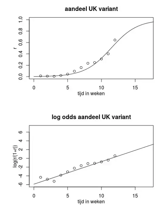
Personally, I always like to think first about what we are modelling before proceeding with the interpretation. In your case, you are modelling the logit-transformed expected proportion at a given x as a function of x. Something like this:

logit(expected proportion) = beta0 + beta1*x 

The expected proportion is the (true) average proportion across all units/subjects in your target population having the same value of x.

If we denote the expected proportion via ep for convenience, the logit transformation is in effect:

logit(ep) = log(ep/(1-ep))

These types of models with a logit link can be interpreted on multiple scales.

On the logit scale, you could just say things like:

Each 1-unit increase in the value of x is associated with a change of b1 points on the logit-transformed value of the expected proportion.

Here, b1 is the estimated value of beta1 from the data. (People talk about points as being units on a logit scale.)

The "odds" scale would be the next possible scale, except that the odds terminology makes more sense with a probability rather than an expected proportion. But that is the scale you would find yourself working with if you exponentiated the value of b1. In other words, exp(b1) would give you the multiplicative factor by which the ratio ep/(1-ep) would change when the value of x increases by one unit. My own view is that ep/(1-ep) does not represent odds per say because ep is not a probability, it is a continuous proportion. So I would just talk about the ratio ep/(1-ep) without calling it odds.

Note that, if you compute (exp(b1) - 1)*100%, you get the % change in the value of the ratio ep/(1-ep) associated with a 1-unit increase in the value of x.

The last possible scale for interpretation of the effect of x is the scale of the expected proportion itself. One can show that:

ep = exp(beta0 + beta1x)/(1 + exp(beta0 + beta1x))

If you plug in the estimated values of beta0 (i.e., b1) and beta1 (i.e., b1) from your model summary output for the quasibinomial regression with a logit link, you get to see how the estimated value of ep (expected proportion) varies with the values of x and can easily visualize that. Of course, on the expected proportion scale, x has a nonlinear effect so you can just qualitatively describe it or just mention whether your study provides evidence that x has a positive nonlinear effect on the expected proportion (if b1 > 0; p-value for testing H0: beta1 = 0 vs Ha: beta1 != 0 reasonably small) or a negative nonlinear effect on the expected proportion (if b1 < 0; p-value for testing H0: beta1 = 0 vs Ha: beta1 != 0 reasonably small).

Answer 2

A model with a logit link function assumes a linear relationship between the logit-transformed variable (log-odds when we speak about logit transformed probabilities) and the predictors.

(Note that this assumption of linearity might be false and it can lead to the piranha problem when we extrapolate too far or with too many combined multiple effects)

Below you see an example image of the relationship with the logit link function.

The image is an example of the fraction of the UK Covid variant as function of time. This is modelled with a logistic function. Then the logit transformed data (the log-odds) are considered linear. (In this particular example you see that the model is not perfect and it is not exactly a straight line)

In the upper image it is the fraction on the y-axis. In the lower image it is the same data and fit but expressed as log-odds on the y-axis.

---

So the fit with a logit function has a linear interpretation in terms of logit transformed data. The coefficients from the output relate to the line in the graph with the logit transformed data on the y-axis.

In terms of the fraction the relationship is non-linear (the upper graph). At different points an increase in the parameter will have a different increase in the fraction. The coefficients will not have a clear/intuitive interpretation in terms of the fraction.