GAM and multiple continuous-continuous interactions/tensor smooths

Question

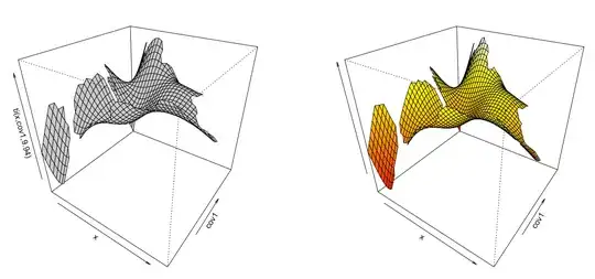
I've looked through multiple previous questions on this topic and I have made some progress understanding continuous/continuous interactions with a GAM, but I still need some help understanding my results and making sure my modeling approach is statistically sound. I'm still very new to modeling with GAMs. I'm using mgcv in R.

I have a principle (nonlinear) relationship of y~s(x)+blocking_var. Now, we're interested in whether/how a number of continuous covariates qualitatively change that relationship. We are not interested in the main effects of those covariates as they will not be real-life causal predictors of y.

All covariates we're interested in are continuous. There may be some collinearity and we suspect nonlinear interactions. Our main predictor and the other covariates are on different units/scales, e.g. normalized counts:julian day, normalized counts:percentage of counts of group A etc.

For an interaction with one additional covariate, I understand I can do y~te(x,cov1) + blocking_var. But, how do I incorporate multiple factors?

My questions are:

1. Do I actually need to use te() instead of s() as in y~s(x,cov1) + blocking_var ?

2. Can I do:

y~te(x,cov1) + te(x,cov2) + te(x,cov3) + blocking_var

or should I create separate models for each interaction I'm trying to test? How would I account for possible influences on the various terms on each other?

3. Do I need to include a separate s(x) term? i.e. y~ s(x)+ te(x,cov1) + te(x,cov2) + te(x,cov3) + blocking_var

4. What is the difference between te() and ti()? That part I'm still not clear about.

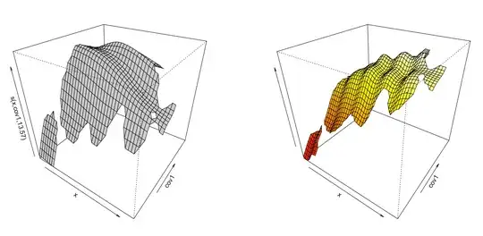
5. I visualized the partial effects with both plot.gam and vis.gam and get vastly different plots depending on how I fit the model between plot.gam and vis.gam. I do not understand why the two ways to plot the model are so different, both among the two plotting functions as well as whether I use s(), te(), or ti().

gam.1<-gam(y~ s(x) + s(x,cov1) +  s(x,cov2) + s(x,cov3) + blocking_var, data=df, method = 'REML')
par(mfrow = c(1,2))
plot(gam.1, select=2, scheme=1, theta=35, phi=32,) 
vis.gam(gam.1, view=c('x', 'cov1'), n.grid=50, theta=35, phi=32, zlab="", too.far=0.1)

gam.2<-gam(y~ s(x) + te(x,cov1) +  te(x,cov2) + te(x,cov3) + blocking_var, data=df, method = 'REML')
plot(gam.2, select=2, scheme=1, theta=35, phi=32,) 
vis.gam(gam.2, view=c('x', 'cov1'), n.grid=50, theta=35, phi=32, zlab="", too.far=0.1)

gam.3<-gam(y~ te(x) + te(x,cov1) +  te(x,cov2) + te(x,cov3) + blocking_var, data=df, method = 'REML')
plot(gam.3, select=2, scheme=1, theta=35, phi=32,) 
vis.gam(gam.3, view=c('x', 'cov1'), n.grid=50, theta=35, phi=32, zlab="", too.far=0.1)

gam.4<-gam(y~ te(x,cov1) +  te(x,cov2) + te(x,cov3) + blocking_var, data=df, method = 'REML')
plot(gam.4, select=1, scheme=1, theta=35, phi=32,) 
vis.gam(gam.4, view=c('x', 'cov1'), n.grid=50, theta=35, phi=32, zlab="", too.far=0.1)

gam.5<-gam(y~ ti(x,cov1) +  ti(x,cov2) + ti(x,cov3) + blocking_var, data=df, method = 'REML')
plot(gam.5, select=1, scheme=1, theta=35, phi=32,) 
vis.gam(gam.5, view=c('x', 'cov1'), n.grid=50, theta=35, phi=32, zlab="", too.far=0.1)

This obviously also has impact on subsequent maximum likelihood tests and whether or not terms/interactions are significant.

Thank you.

Edit: Following the really helpful reply by Isabella, I wanted to update my post with some more information regarding my specific data/modeling needs.

We know that:

y~s(x)
y~s(cov1)
x~s(cov1)

Therefore, x and cov1 are highly collinear. For our specific question, we're only interested in the relationsship y~x. This relationship is actually almost linear (it's quadratic), but for modelling purposes we still chose a GAM due to probable nonlinear interactions. We are intersted in how that simple y~xrelationsship changes qualitatively due to the impact of the other factors.

Cov1 is a temporal variable.

Cov2 and Cov3 are derivates of x, i.e they're not independent of x. They are proportions of specific groups of x per x (e.g. %females of counts x). There may be some slight collinearity, but if so it's not strong. Cov2 and Cov3 are not practical/causal predictors of y, therefore I should not include them as separate fixed effects, as far as I understand it.

We are not trying to find the best possible model describing our data. We're trying to describe qualitative modifications of covariates on our simple regression that is our primary interest.

Given those information, do I conclude correctly that the best approach is to use all te() terms?

(a) y~te(x,cov1) + te(x,cov2) + te(x, cov3) + blocking_var

or should I do something like

(b) y~te(x,cov1) + ti(x,cov2) + ti(x, cov3) + blocking_var ?

If b, is it sufficient to include te(x,cov1) instead of an additional ti(x) when using ti() for the other two covariates? As mentioned above, cov2 and cov3 should not be included as fixed effects; at least I wouldn't understand the practical (in my case biological) logic behind it.

Edit2: Adding another question.

6. How do I interpret maximum likelihood ratio tests with te()? With GLM with interactions, when I run a Type II anova, I will get p values for the fixed main effects and the interaction. A significant interaction means my significant main effect 1 isn't independent of value/factor of covariate 1.

With te(), I don't have separate main effects. What does a significant te() mean? How do I interpet this? I would assume I would interpet results from y~ti(x) + ti(x,cov1) the same as in a GLM. But how about y~te(x,cov1). Does it only mean x isn't independent of cov1, but what does it tell me about my response? How will I know which are my main predictors of y?

Answer 1

Nice question! Here are some hints to get you started. Your questions are not numbered well (question 2 appears twice), so you may want to renumber them to avoid confusion.

Question 1

The general rule is that you would use an isotropic smooth s(x, cov1) if x and cov1 had the same units and you would use an anisotropic smooth te(x, cov1) if x and cov1 had different units. See Simon Wood's slides at https://www.maths.ed.ac.uk/~swood34/talks/gam-mgcv.pdf.

An isotropic bivariate smooth would use the same degree of smoothness along both of its dimensions; an anisotropic bivariate smooth would use different degrees of smoothness along its two dimensions.

Question 2

Yes, you can include all 2-way interactions between x and your 3 covariates in the same model using te() terms (and presumably test whether you actually need all of them or just some of them in the model).

In principle, you can fit all of these models to your data:

y ~ te(x,cov1) + blocking_var

y ~ te(x,cov2) + blocking_var

y ~ te(x,cov3) + blocking_var

y ~ te(x,cov1) + te(x, cov2) + blocking_var

y ~ te(x,cov1) + te(x, cov3) + blocking_var

y ~ te(x,cov2) + te(x, cov3) + blocking_var

y ~ te(x,cov1) + te(x, cov2) + te(x, cov3) + blocking_var

and compare them to see which one receives most support from your data. When comparing them, make sure all models use the same number of observations so that the comparison is fair (which would not be the case if some of your covariates included missing data) and are fitted using the option method = "ML", as clarified by Dr. Gavin Simpson in his comments.

The model comparison can rely on comparing the AIC or BIC values, the adjusted R squared, the model diagnostics, etc.

Note that if it is important to control for all 3 covariates, cov1 through cov3, in your model, you would consider only the last of the above models and forego the model comparison.

Question 3

The help file for the te function states the following:

"te produces a full tensor product smooth, while ti produces a tensor product interaction, appropriate when the main effects (and any lower interactions) are also present."

There are differences between te and ti with respect with how you specify interactions. For example, you would specify a 2-way smooth interaction between x and cov1 like this using te:

y ~ te(x,cov1) + blocking_var

and like this using ti:

y ~ ti(x) + ti(cov1) + ti(x, cov1) + blocking_var

The ti formulation assumes that you can split the effect of x on y into an effect purely due to x (which will be captured by ti(x)) and an effect due to the combination of x and cov1 (which will be captured by ti(x, cov1)). The te formulation implies that such a split may not necessarily be possible (though you could check to see if it is).

See Dr. Gavin Simpson's answer on this forum: R/mgcv: Why do te() and ti() tensor products produce different surfaces?.

Note that an alternative way to formulate the model below which includes ti terms:

y ~ ti(x) + ti(cov1) + ti(x, cov1) + blocking_var

is this:

y ~ s(x) + s(cov1) + ti(x, cov1) + blocking_var

Indirectly, this suggests that you should NOT include s(x) and/or s(cov1) in a model of the form:

y ~ te(x, cov1) + blocking_var

Addendum

Collinearity has an extension to GAM models which is called concurvity. See the help for the concurvity() function in the mgcv package for details on how to check for the presence of concurvity in your model(s).

With cov2 and cov3 being defined as derivatives of x, you might need to worry about a phenomenon called mathematical coupling.

Answer 2

Q1

Almost invariably yes, you should use te() for smooth interactions. The only situation where you might not want to do that is where you are smoothing in multiple dimensions but everything is in the same units, like space. In such circumstances an isotropic smooth may make sense via s().

Q2

My personal belief is that you should fit the full model and do any required inference on that full model. As you have the same term appearing in multiple smooths, you should probably decompose those smooths into main effects and interactions via:

y ~ s(x) + s(cov1) + s(cov2) + s(cov3) + ## main effects
  ti(x,cov1) + ti(x,cov2) + ti(x,cov3) + ## interactions
  blocking_var                           ## other stuff

If you want to do selection on that model, you could add select = TRUE to add an extra penalty to all smooths such that they can be penalised out of the model entirely, or change the basis to one of the shrinkage smooths via the bs argument to s(), te() etc., e.g. s(x, bs = 'ts') for shrinkage thin plate splines and te(x,z, bs = c("cs", "ts")) for a tensor product of x and z with a cubic regression shrinkage spline marginal basis for x and a shrinkage thin plate spline marginal basis for z.

If you are going to fit and compare nested models explicitly, make sure you use method = "ML" because the corrections used to compute the REML uses information from the fixed effects and if you models include different fixed effects terms — and the ones in the example do — you re making different corrections to the likelihood to compute REML and that renders the REML likelihoods incomparable.

Q3

You include single terms with s() and pure interactions with ti(). While {mgcv} will try to make the models identifiable if you do things like s(x) + te(x, z), it is better if you can decompose the effects manually as that will give you the most stable fit (by "that" I mean answer to Q2).

Q4

te(x, z) includes both the smooth main effects of x and z, plus their smooth interaction. ti() is just the pure smooth interaction of x and z.

If you are familiar with R's linear modelling formulas, then

• te() is like x*Z or x + z + x:z if you want to write it all out
• ti() is like X:Z only

Q5

plot.gam() is producing partial effect plots for each term separately. vis.gam() is showing model fitted values (expectations of the response, $E(\hat{y})$). The reason you are will be seeing very different plots is that in the example from [so] (y ~ s(x) + te(x, cov1) + other_stuff) with plot.gam() for the tensor product you are just getting a plot of that tensor product smooth. When you use vis.gam() varying x and cov1 you are getting a plot of the expected response from the whole model s(x) + te(x, cov1) + other_stuff, when you vary input values x and cov1 while holding other_stuff at representative (or user supplied) values.

Q6

Think of the te() as a single term that just happens to include both smooth main effects and smooth interactions. Hence in the anova() or similar output, you are just setting this entire term to 0 and comparing the fits. This is not like a model with x * z where that actually implies three terms x + z + x:z and say you are testing x:z, you are just setting this pure interaction term to zero in anova().

If you want an ANOVA-like decomposition then use s(x) + s(z) + ti(x, z) as you will now have separate functions for the three things specified. Now you can compare that model with s(x) + s(z) by setting the ti() term to zero so you get the proper nesting.

A significant te() just means that the estimated smooth function differs from a flat surface or constant function.

You could interpret that smooth by visualising it and see how the expected value of the response varies over the surface. If you want to do more formal inference, you can do the ANOVA-like decomposition of the te(x,z) term into s(x) + s(z) + ti(x,z) and now you have a term that comes with a formal test of whether the pure interaction (for example) is consistent with a flat or constant functions.

However, you should note that the te(x,z) and s(x) + s(z) + ti(x,z) models are not strictly equivalent; the latter has more smoothness parameters to estimate — IIRC the te() one would have 2 smoothness parameters and the s(x) + s(z) + ti(x,z) version 4 smoothness parameters.

The reason we would prefer a model specification like this

y ~ s(x) + s(cov1) + s(cov2) + s(cov3) + ## main effects
  ti(x,cov1) + ti(x,cov2) + ti(x,cov3) + ## interactions
  blocking_var                           ## other stuff

is that if you have say two terms te(x,z) + te(x,v) then the basis for te(x,z) contains functions for x that overlap with basis functions for x from the other te(x,v) term. What this means is that you are effectively including the same variables in the model twice and you can't uniquely identify such duplicated terms — adding a constant to one can be offset by subtracting the same constant from the other and as the constant could be any number you have an infinity of models that are all the same. {mgcv} will try to remove these rank deficiencies from the model matrix, but it will do so by making the te() terms difficult to interpret because one of them will have had some of the main effects of x removed from it.

Hence it is better to manually decompose the fit into main effects and interactions, plus doing so should result in a model that is much easier to fit and hence the fitting process should be stable.

Finally, I prefer to use s(x) + s(z) + ti(x,z) even though you can use ti(x) + ti(z) + ti(x,z) because a ti means a tensor interaction and it is just confusing to think of a tensor interaction of a single variable — there is no interaction going on — plus at one point Simon indicated that he was going to remove the ability to fit tensor products of single terms, including in ti(), though he seems to have removed that comment from the changelog since.