I'm not a statistician, but need to use these clever tools to analyse some data I have.
I have a really simple dataset to analyze (see below. cases=disease counts, pop=total number of subjects sampled per year), but can't seem to settle on the most appropriate model to use.
It is count of a disease across different years.
I am interested in studying the change in disease counts over the study period (2000-2008) and to see if this change is 'significant'.
I am under the impression that poisson regression would be appropriate to model how the disease count changes over time. The disease count is its prevalence - therefore accounting for old and new cases in a year. Therefore, my data violates the assumption that the counts are independent of each other as they are not. Counts in 2001 for example may have been from the same individuals sampled in 2000.
'data.frame':   9 obs. of  4 variables:
 $ year      : int  2000 2001 2002 2003 2004 2005 2006 2007 2008
 $ cases     : int  76 103 110 129 129 135 144 130 147
 $ pop       : int  3766 4012 3993 4111 4086 4100 4060 4132 4084
I have tried performing poisson regression using glmer() by specifying 'year' as a random effect to account for clustering of cases between years, but it gives me this error message:
boundary (singular) fit: see ?isSingular
Maybe it's because my dataset is too small??
My question is quite simply how do I use poisson regression to account for repeated measures in this case?
If I were to assume independence of observations/counts, using poisson regression in glm() gives me some interpretable results showing that the increase in counts over time is statistically significant. Not sure if i can trust these results if I haven't accounted for repeated measures...
Any help, comments are appreciated!
I have added a bit more detail - please check if I am doing this correctly for the type of data I have. Here it is:
> new.prevalence.data
  year cases  pop   logpop
1 2000    60 3700 8.216088
2 2001    70 4000 8.294050
3 2002   100 3990 8.291547
4 2003   130 4100 8.318742
5 2004   140 4086 8.315322
6 2005   140 4100 8.318742
7 2006   167 4060 8.308938
8 2007   170 4132 8.326517
9 2008   175 4084 8.314832
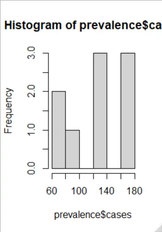
Distribution of counts looks like this

poisson.model.rate<-glm(cases~year+offset(logpop), family=poisson, data=new.prevalence.data)

    > summary(poisson.model.rate)

Call:
glm(formula = cases ~ year + offset(logpop), family = poisson,
    data = new.prevalence.data)

Deviance Residuals:
     Min        1Q    Median        3Q       Max
-1.81701  -1.37797   0.08085   1.02010   1.76332

Coefficients:
              Estimate Std. Error z value Pr(>|z|)
(Intercept) -229.96091   23.70549  -9.701   <2e-16 ***
year           0.11301    0.01182   9.557   <2e-16 ***
---
Signif. codes:  0 ‘***’ 0.001 ‘**’ 0.01 ‘*’ 0.05 ‘.’ 0.1 ‘ ’ 1

(Dispersion parameter for poisson family taken to be 1)

    Null deviance: 107.55  on 8  degrees of freedom
Residual deviance:  13.72  on 7  degrees of freedom
AIC: 77.391

Number of Fisher Scoring iterations: 4
My dispersion parameter here is 1.96. Therefore I've proceeded to use the quasipoisson model:
Call:
glm(formula = cases ~ year + offset(logpop), family = quasipoisson,
    data = new.prevalence.data)

Deviance Residuals:
     Min        1Q    Median        3Q       Max
-1.81701  -1.37797   0.08085   1.02010   1.76332

Coefficients:
             Estimate Std. Error t value Pr(>|t|)
(Intercept) -229.9609    33.0696  -6.954 0.000220 ***
year           0.1130     0.0165   6.851 0.000242 ***
---
Signif. codes:  0 ‘***’ 0.001 ‘**’ 0.01 ‘*’ 0.05 ‘.’ 0.1 ‘ ’ 1

(Dispersion parameter for quasipoisson family taken to be 1.946079)

    Null deviance: 107.55  on 8  degrees of freedom
Residual deviance:  13.72  on 7  degrees of freedom
AIC: NA

Number of Fisher Scoring iterations: 4
Does anyone see a problem with using this model to reach the conclusion that prevalence increases with time and that this increase is significant? i.e. a 1 unit increase in year results in a multiplicative increase by a factor of exp(0.113) that is statistically significant (p<0.05)?
Thank you