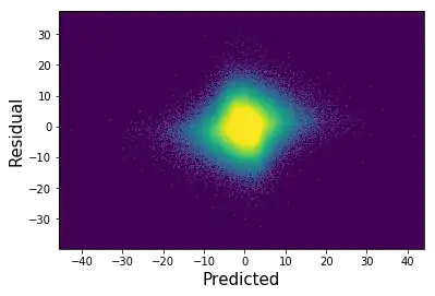
Let's agree on notation: $Y$ is a target variable, $Y'$ is a fitted model output. Then, $Y - Y'$ is a residual term.
Indeed one expects to see on the plot of target vs. fitted to align with the line of the form
$$Y' = Y$$
The spread of data points around this line indicates how much information was not accounted for in the model. So, your expectation is correct. I am sorry I have made misleading comments on this point.
The summary looks OK.
You got a significantly large slope, and a non significant intercept. So the intercept is zero.
R^2 is high enough, and it is definitely more than zero in statistical sense.
$$Y = 0.623 * X$$ is effectively your model.
To your charts:
My advice is to plot these data as a heatmap, and zoom-in on an area with the highest density. Then you should observe the dense cloud which forms a majority of your data goes in line with the diagonal. If you dont's see that that means your model does not have enough independent variables / chosen IV are weakly associated with the target.
Residuals vs. fitted. It should not have a trend, nor linear nor nonlinear, so that variation of $Y - Y'$ is equal for all $Y'$. I could say your plot looks OK.
I don't say you could improve the fit by weithing cases. That, in turn, could change the shape of the tails in distribution, but make it worse in the middle. Better try different candidate independent variables, if you have a choice, of course.
What else to look at:
A prob. density for the residuals. Ideally, but not necessary, they should be close to a normal shape. Normally distributed residuals tell us that the model contains all the infomative regressors about the target, leaving so called "measurements errors" only, which are expected to be normally distributed.
Finally, this is a possible duplicate of: Interpret regression model actual vs predicted plot far off of y=x line
and Interpret if residuals are "close enough" to a normal distribution

