Law of the norm of the empirical mean of uniforms on the sphere?

Question

Let $U_1,\dots,U_n$ be i.i.d, uniform on the euclidean sphere on $\mathbb{R}^d$ that we denote $S^{d-1}$. I am searching for the law of $$M=\left\|\frac{1}{n}\sum_{i=1}^n U_i \right\|.$$

Attempts:

I don't know if it is possible to determine the law exactly, I need a lower bound on $M$ so I tried U-Statistics deviation bounds but the bound I obtained is not sufficient, I want to be able to say that with some small probability, $M$ is greater than $\sqrt{\lambda/n}$ for some $\lambda\le n$ (with U-stats I am limited to $\lambda \le 1$).

• U-Stat approach: if we take the square, we obtain $$M=\left\|\frac{1}{n}\sum_{i=1}^n U_i \right\|^2 = \frac{1}{n} +\frac{1}{n^2}\sum_{i \neq j} \langle U_i, U_j\rangle .$$ For one individual term $\langle U_i, U_j\rangle$, we know what is the law (related to Distribution of scalar products of two random unit vectors in $D$ dimensions and https://math.stackexchange.com/questions/2977867/x-coordinate-distribution-on-the-n-sphere) but these terms are not independent hence taking the sum is not easy.

• Another possibility is to write that $$M=\left\|\frac{1}{n}\sum_{i=1}^n U_i \right\|^2 = \frac{1}{n^2} +\frac{2}{n^2}\langle U_1, \sum_{i=2}^n U_i\rangle + \left\|\frac{1}{n}\sum_{i=2}^n U_i \right\|^2 .$$ then, by independence of the $U_i's$, we have $$\mathbb{P}\left(\left\|\frac{1}{n}\sum_{i=1}^n U_i \right\|^2 \le x\right)=\mathbb{E}\left[ \mathbb{P}\left(\frac{1}{n^2} +\frac{2}{n^2}\langle U_1, \sum_{i=2}^n U_i\rangle + \left\|\frac{1}{n}\sum_{i=2}^n U_i \right\|^2 \le x\big| U_2,\dots, U_n\right)\right] $$ and we know that the law of $(1+\langle U_1, \sum_{i=2}^n U_i\rangle)/2$ is a $Beta(d/2, d/2)$ distribution (conditionally on $U_2,\dots,U_n$) hence, $$\mathbb{P}\left(\left\|\frac{1}{n}\sum_{i=1}^n U_i \right\|^2 \le x\right)=\mathbb{E}\left[ F_{Beta(d/2,d/2)}\left( \frac{n^2x}{4}+\frac{1}{4}- \frac{1}{4}\left\|\sum_{i=2}^n U_i\right\|^2 \right)\right] $$ and this, I want to find an upper bound but I don't think I will succeed with this line of thought.

Answer 1

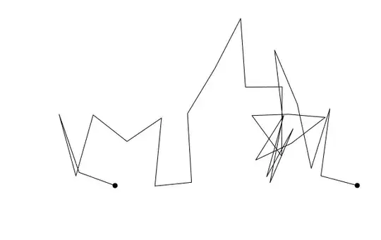
Similarity with a rubber band model.

This problem got me to think of the model for a 'rubber band' (See for instance wikipedia or section 3-7 in Herbert B. Callen's thermodynamics and an introduction to thermostatistics).

With a bit of hand waving:

• consider the distribution of only one axis/component of the $U_i$ (the marginal distribution along a single axis)
• approximate this with a normal distribution (the approximation becomes more accurate for larger $n$ and also for larger $d$)
• because the distribution needs to be spherically symmetric we assume the other components to be identical and independently distributed.
• The squared length will be the sum of $d$ squared normal distributed variables.

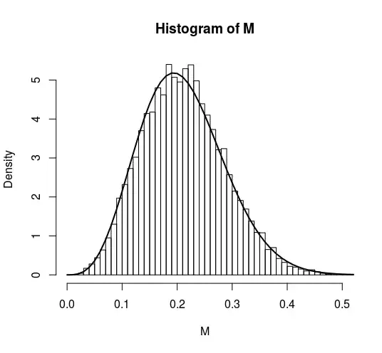
Then the distribution of $M$ is approximately a scaled $\chi$ distributed variable with $d$ degrees of freedom. The scaling factor is $1/\sqrt{dn}$

To know the scaling we need to know the variance of the distribution of the component. The contributions of each $U_{i}$ follow some sort of beta distribution (it is only the projection of $U_{i}$ that matters)

$$f(x) \propto (1-x^2)^\frac{d-3}{2} \quad \text{for $-1 \leq x \leq 1$}$$

or with $t = x^2$

$$f(t) \propto t^\frac{1}{2}(1-t)^\frac{d-3}{2}\quad \text{for $0 \leq t \leq 1$}$$

This means that the mean of $T$ or the variance of $X$ is equal to $1/d$ (the mean of a beta distribution with $\alpha = 1/2$ and $\beta = (d-1)/2$). For the mean of $n$ of those variables, you get that the variance is $1/(dn)$.

Simulation

Below is an example for the case of $n=20$ and $d=4$

This is computed with the following r-code:

n = 20
d = 4

### sample from sphere
simsphere <- function(d) {
  x <- rnorm(d)
  x <- x/sqrt(sum(x^2))
  return(x)
}

### add 'n' times U and compute absolute value
getM <- function(n,d) {
  xv <- replicate(n,simsphere(d))
  vector <- rowSums(xv)
  norm <- sum(vector^2)^0.5
  return(norm/n)
}
  
### chi distriution
dchi <- function(x,nu) {
  x^{nu-1}*exp(-1/2*x^2)/(2^((nu/2)-1)*gamma(nu/2))
}
dchi <- Vectorize(dchi)

### simulate and plot histogram
M <- replicate(10^4, getM(n,d))
hist(M, breaks = seq(0,5,0.01), freq = 0, xlim = c(0,0.5))

### add approximation based on chi distribution
v = 1/d/n
ms <- seq(0,10,0.01)
lines(ms,dchi(ms/sqrt(v),d)/sqrt(v), col = 1, lwd = 2)

Answer 2

Densities of short uniform walks in higher dimensions could be relevant. It discusses random walks with $n$ steps each of length $1$ in $\mathbb{R}^d$, where each step is taken in a uniformly random direction.

Theorem 2.1 states that the probability density function of the distance to the origin in $d \ge 2$ dimensions after $n \ge 2$ steps is, for $x \gt 0$,

$$p_n(\nu; x) = \frac{2^{-\nu}}{\nu!}\int_0^\infty (tx)^{\nu+1}J_v(tx)j_\nu^n(t)\:dt$$

Where:

• $\nu = \frac{d}{2}-1$
• $J_\nu$ means the Bessel function of the first kind
• $j_\nu(x) = \nu!(\frac{2}{x})^\nu J_\nu(x)$ is the "normalized Bessel function of the first kind"

The norm of the mean of the steps is just the final distance from $0$ divided by $n$. So you could theoretically plug $x = ny$ into the formula to get the value of the pdf you care about at $y$. But looks like it could be computationally difficult. (Theorem 2.10 apparently gives a "computationally more accessible" expression for the pdf.)

Answer 3

I'm not sure if you want an upper or lower bound. You mention both in the question. The easiest way to get a very loose upper bound on this problem is to use Markov's inequality. Just in case it's been overlooked.

$$M=\left\|\frac{1}{n}\sum_{i=1}^n U_i \right\|.$$

$$P\left(M \ge \sqrt{\frac{\lambda}{n}}\right) \le \sqrt{\frac{n}{\lambda}}E[M]$$ by Markov's inequality.

Then by Jensen's inequality, $$E[M] < \sqrt{E[M^2]}.$$

So, the final bound is $$P\left(M \ge \sqrt{\frac{\lambda}{n}}\right) \le \frac{\sqrt{\sum_i \sum_j E\left[ \langle U_i,U_j \rangle \right]}}{\sqrt{\lambda \ n}}.$$

Finding the expectation of the inner product of two independent $U_i$ and $U_j$ shouldn't be too hard. Again, this will be a very loose bound, but it's better than no bound (sometimes).