one example of LDA and max number of features

Question

as i read the following post:

Sources' seeming disagreement on linear, quadratic and Fisher's discriminant analysis

and see the following note:

any where on google we see number of reduction is number of classes minus one. but here how this value reached? i.e: $X-1$

Important: $X << P $ in this example.

Update 1: I think the answer is # of classes minus one but at most we can use as much as training samples in LDA (no restriction up to $X-1$).

Update 2: I see in this Strange Link In a nutshell, the goal of a LDA is often to project a feature space (a dataset $n$-dimensional samples) into a smaller subspace $k$ (where $k \leq n-1 $))...

Update 3:

In Page 27 of this book tell us $n$ classes and $k$ features we get $k-1$ features by LDA.

Answer 1

About linear discriminant analysis

A classical example of least discriminant analysis is R.A. Fisher's 1936 article "The use of multiple measurements in taxonomic problems". This is based on the iris dataset and easily plotted.

### load library 
### with Edgar Anderson's Iris data set 
### and the lda function
library(MASS)

### Perform lda
lda <- lda(Species ~ Sepal.Length + Sepal.Width + Petal.Length + Petal.Width  , data = iris)

### Compute the discriminant
predict(lda)

### Plot histogram with result from first discriminant
plot(lda, dimen=1, breaks = seq(-10,10,0.5))

### Plot histogram with only one variable
layout(matrix(1:3,3))
hist(iris$Sepal.Length[iris$Species == "setosa"], breaks = seq(3,9,0.25), 
     main = "", xlab = "group setosa", freq = 0)
hist(iris$Sepal.Length[iris$Species == "versicolor"], breaks = seq(3,9,0.25), 
     main = "", xlab = "group versicolor", freq = 0)
hist(iris$Sepal.Length[iris$Species == "virginica"], breaks = seq(3,9,0.25), 
     main = "", xlab = "group virginica", freq = 0)

Result from first linear discriminant

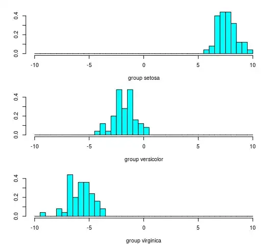
Result from a single variable (sepal length)

The idea from Fisher was to use a linear combination of the variables such that the distance between the classes is larger. This distance is considered relative to the variance of the groups. (To see more about this, consider this question: When is MANOVA most useful )

When parameters > samples

So, the intuition behind LDA is to find a linear combination of parameters for which the in-between distance/variance of the groups is larger than the within distance/variance of the groups.

When you have more parameters than the sample size, then you will be able to find a perfect linear combination. One for which the within distance is zero.

This linear combination can be found by finding the linear combination of parameters for which the linear combination in one class equals zero and in the other class equals one.

This relates to solving a linear regression problem

$$Y = \beta X$$

Where $Y$ is a column with ones and zeros depending on the class, $X$ is a matrix with the features, and $\beta$ are coeffients to be found.

This problem is overdetermined when the number of features is larger than the number of samples. This means that you will be able to find many linear functions of the features for which the one class equals zero and the other class equals one (as long as there are no different class members with the exact same features).

The number of features that you need is similar to the number of features that you need to fit exactly a regression problem. Which is $X-1$. For example, if you have two data points then a straight line, a function of only one feature (and a function of two parameters, because besides the slope the intercept is included as well), will fit perfectly through the points.

So $x-1$ features will be sufficient to find a perfect solution to the LDA problem

Regularization

So, when the number of features is larger than the sample, then the problem is similar to a regression problem.

For this over-determined case, you can say that $X-1$ features are sufficient, but it is not the only solution. The exact answer will be dependent on how you weigh the different solutions. You can do this in several ways. Regularization is one way to do it. In the case that the problem is solved with Lasso regression or stepwise regression (which add regressors/features in steps, building up a solution starting with zero regressors), then I can imagine that the limit is $x-1$ features. In the case that the problem is solved with ridge regression (which uses all regressors/features from the start) then this is not the case.