1

Suppose that I simulate four different Ornstein-Uhlenbeck processes $X^1, \ldots, X^4$ using this example code (Euler-Maruyama).

Using this code, it should be possible to ensure that the $X^1, \ldots, X^4$ are

  • all stationary, by sampling their initial value from their respective stationary distributions;
  • mutually statistically independent, by using different random seeds for their respective implementations.

However, when testing the $X^i$ for independence by using independence tests such as dHSIC (which should be applicable as the $X^i$ are stationary), the null hypothesis of mutual independence is typically rejected with extremely low $p$-value.

Do you have an idea where my mistake is (and how to correct it)?

Edit: Stationarity and independence of the $X^i$ are 'ensured' (I would think) as follows:

  • For the stationarity of the $X^i$, we choose the initial condition according to the stationary distribution of the Ornstein-Uhlenbeck process, i.e. if $X^i$ has the coefficients $(\theta_i, \mu_i, \sigma_i)$ then we set $X^i(0)\sim\mathcal{N}(\mu_i, \sigma_i^2/(2\theta_i))$ for each $i=1, \ldots, 4$. In the given code, this corresponds to setting y_init = np.random.normal(loc=mu_i, scale=sigma_i**2/(2theta_i)).

  • The independence of $X^1, \ldots, X^4$ should be automatic as each $X^i$ is generated with a different random seed.

  • The hypothesis test for mutual independence of the $X^i$ is conducted by applying the function $\texttt{dhsic.test()}$ from the $\texttt{R}$-package $\texttt{dHSIC}$ to the data matrices $\mathfrak{R}_1, \ldots, \mathfrak{R}_4$ defined as

    R_i = Xi.reshape(n,b),

    i.e. for each $i=1, \ldots, 4$, the realisations Xi of the time series $X^i$ are 'chopped' into n-many rows which are treated as realisations of the random vector $R_i:=(X^i(1), \ldots, X^i(b))$ (with b some fixed length). The independence of the $X^i$ is then tested for by testing the independence of the random vectors $R_1, \ldots, R_4$ via

    dhsic.test(list(R_1, R_2, R_3, R_4), method="permutation", kernel=c("gaussian"), B=1000).

rmcerafl
  • 45
  • 5
  • Could you add some code and plots, and specify more clearly how you make the comparison/test. For instance, one way that you can get dependence is when you do not select a random starting point. Are you doing this or not (the code in your example is using a fixed y_init=0)? There might be more, but it is difficult to see. – Sextus Empiricus Oct 13 '20 at 16:33
  • Thank you for your comment, @SextusEmpiricus. I will edit the question now to address these points. – rmcerafl Oct 13 '20 at 16:45
  • Can you provide more information about your implementation (in order to see more than just the point with the init value). I am not sure how the dHSIC works but the OU-process should give independent time series that don't give problems with independence tests. So there is probably something with your code. A plot of some graphs with the time series, or a table, may help others to verify your results. – Sextus Empiricus Oct 13 '20 at 17:09
  • @SextusEmpiricus : I'm currently preparing the edit, but just in general: You don't see that there should be anything wrong with dividing the time-series-data according to `X_i = Xi.reshape(nobs,bdim)` (so that the rows are realisations of dependent vectors of dimension `bdim`) and provide these realisations as an input to statistical dependence tests (such as stats.spearmanr() for instance)? (I suppose that the fact that the rows of `X_i` are not iid will be mitigated by the stationarity of $X^i$ (and it being 'mixing' in some sense)?) – rmcerafl Oct 13 '20 at 17:28
  • I am not so fluent in python, and unsure what nobs means. You mean that you did not simulate 4 independent time-series but instead, you have cut up a single process in pieces and compared the pieces from the same time-series? These pieces will be dependent and only for sufficiently long time delays will it become negligible. Stationarity does not mean lack of autocorrelation. – Sextus Empiricus Oct 13 '20 at 17:38
  • Thanks, @SextusEmpiricus. Sorry for the confusion: In the above, nobs is just a variable to denote the 'number of observations' (per batch) (could have called it just n or anything else). I did simulate 4 independent time series, and each one of them (which, say, consists of N=1000 realisations) I chopped into `nobs`-many batches of length `bdim` (say each `Xi` is chopped up into `nobs=200` many batches of length `bdim = 5` each). I then tested independence of the $X^i$ by applying an independence test to the 5 batches (i.e. random vector of length 5 for which 200 realisations are given). – rmcerafl Oct 13 '20 at 17:50
  • (This is because all of the independence tests that I'm aware of are only applicable to random vectors of some finite dimension, so that for each $X^i$ I had to cut our one such random vector $R_i = (X^i_{t_0},\cdots, X^i_{t_{\mathrm{bdim}}})\in \mathbb{R}^{\mathrm{bdim}}$ out of $X^i$ and treat the full realisations of $X^i$ as realisations of this $R_i$.) – rmcerafl Oct 13 '20 at 17:55
  • @SextusEmpiricus But in case this just adds to the confusion, please don't feel bothered by all this. I already appreciate your help so far! – rmcerafl Oct 13 '20 at 18:00

1 Answers1

1

Reproduction of your problem

I can reproduce your result with the following R code:

library(dHSIC)

######## function to generate a time series
### for the Ornstein-Uhlenbeck processes using Euler-Maruyama method
### time    = length of time interval of time series
### n       = number of points in time series
### mu      = drift term (long term mean level)
### theta   = speed of reversion
### sigma   = noise level
#######

timeseries <- function(time,n,mu,theta,sigma) {
  # differential equation
  # dX = theta(\mu-X) dt + sigma dW
  
  ### initialization x[1]
  ###  
  ###  Var(x) = Var(x) (1-theta*dt) + sigma^2*dt
  ###  Var(x) =  sigma^2/theta
  x <- rnorm(n = 1, mean = mu, sd = sqrt(sigma^2/theta)) 
  dt <- time/n
  
  #### add new x[i+1] 
  for (i in 1:n) {
    ### compute next value
    xlast <- tail(x,1)
    xnew <- xlast + theta*(mu-xlast)*dt + sigma * rnorm(n = 1, mean = 0, sd = sqrt(dt))
    
    x <- c(x,xnew)   ### add new value to the array
  }
  x
}

#### compute 4 time series
set.seed(1)
t <- seq(0,1,1/1000)
x1 <- timeseries(1, 1000, 0, 10, 2)
x2 <- timeseries(1, 1000, 0, 10, 2)
x3 <- timeseries(1, 1000, 0, 10, 2)
x4 <- timeseries(1, 1000, 0, 10, 2)

### place in matrix form (does not need to be multiple columns)
m1 <- matrix(x1,ncol = 1)
m2 <- matrix(x2,ncol = 1)
m3 <- matrix(x3,ncol = 1)
m4 <- matrix(x4,ncol = 1)

### perform independence test
dhsic.test(list(m1,m2,m3,m4), method="permutation", kernel=c("gaussian"), B=1000)

### plot the time series
plot(t,x1,type = "l", ylim = c(-1.5,1.5))
lines(t,x2, col = 2)
lines(t,x3, col = 3)
lines(t,x4, col = 4)

This gives a p-value of 0.00990099 and the time series look as following:
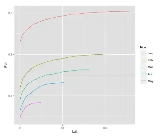
example image of four curves

Explanation: effective degrees of freedom

I do not know much of the details of the dHSIC method (I still need to read through the article). However, we can already argue that in general methods for independence might underestimate the p-value.

For instance, a test for the correlation coefficient, cor.test(x1,x2, method = "pearson"), does also give very low p-values.

The reason is that the time series have auto-correlation. You can see this for instance in the image above where on the right between 0.8 and 1 seconds the red, black and blue curves are sort of stuck near -0.5.

However, many tests for independence are assuming that the values within the time series are not correlated. The influence that this has is in the effective degrees of freedom.

If you have correlated measurements instead of independent measurements, then you are gonna get more often a high correlation between time series due to random fluctuations.

Intuition with a simplified example: Imagine the following two extreme situations.

  • We have two samples $X_i$ and $Y_i$ of size $n=1000$.

    Each $X_i$ and $Y_i$ is independent:

    $$X_i, Y_i \sim N(0,1)$$

    This gives a table like:

    i     X       Y 
    1    -2.05    0.17
    2    -0.86    1.56
    3    -0.39   -0.08
    4     0.09    1.05
    5     0.18    1.84
    ...   ...     ...
    1000  0.19   -1.26
    
  • We have two samples $X_i$ and $Y_i$ of size $n=1000$.

    Each block of 100 samples is equal. $X_i = \mu_{X,j}$ and $Y_i = \mu_{Y,j}$. Where $j = \lfloor i/100 \rfloor$.

    The values of the blocks $\mu_{X,j}$ and $\mu_{X,j}$ are independent:

    $$\mu_{X,j}, \mu_{Y,j} \sim N(0,1)$$

    This gives a table like:

    i     X       Y 
    1    -2.05    0.17
    2    -2.05    0.17
    3    -2.05    0.17
    4    -2.05    0.17
    5    -2.05    0.17
    ...   ...     ...
    998   0.19   -1.26
    999   0.19   -1.26
    1000  0.19   -1.26
    

This latter example has still time series that are independent of each other. The ten values $\mu_{X,j}$ and $\mu_{Y,j}$ are independent. However, the testing assumes that the sample consists of 1000 independent realizations instead of 1000 correlated realizations. This has an influence on the sample distribution of the correlation coefficients (or other statistics that relate to independence) and on the computation of related p-values.

There will always be some correlation due to random fluctuations. These random fluctuations are different for ten values than for thousand values. The time series with correlated values are a lot like that. The auto-correlation has an effect on the random fluctuations in the correlation between different time-series. These random fluctuations are assumed to be lower when the assumption is that all 1000 rows/measurements are independent.

See also the difference in the time series when we look at the original sample or at a completely shuffled sample:

In the first/upper graph you see that the time series have a tendency to occassinaly move along with each other. That is due to random behaviour. However, the test assumes a much more extreme random behaviour and that is the behaviour in the second/lower graph which is for completely shuffled curves.
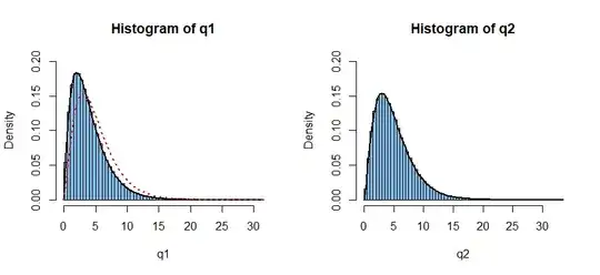
example of shuffling

plot(t,x1,type = "l", ylim = c(-1.5,1.5), xlim = c(0.85,0.95), main = "original sample")
lines(t,x2, col = 2)
lines(t,x3, col = 3)
lines(t,x4, col = 4)


plot(t,sample(x1),type = "l", ylim = c(-1.5,1.5), xlim = c(0.85,0.95), main = "shuffled sample")
lines(t,sample(x2), col = 2)
lines(t,sample(x3), col = 3)
lines(t,sample(x4), col = 4)
Sextus Empiricus
  • 43,080
  • 1
  • 72
  • 161
  • Thank you very much for your excellent answer; this has been very enlightening! – rmcerafl Oct 14 '20 at 12:35
  • Thanks again! Given your comment about the shuffling: Would you expect the independence test to perform more accurately if each $X^i$ would be subjected to a random shuffling prior to applying the test? (Assuming that the random shufflings are statistically independent.) – rmcerafl Oct 14 '20 at 14:09
  • 1
    @rmcerafl yes that would influence the independence test (but also if the time series are dependent it will destroy their dependence). This random shuffling is what the dHSIC function does to compute/estimate the sample distribution of the statistic given the null hypothesis. – Sextus Empiricus Oct 14 '20 at 14:44
  • 1
    I've got one last question on this, if you're interested: In your above application of dhsic.test() you seem to test the independence of the *scalar* variables $X^1_t, \ldots, X^4_t$ (for a fixed $t$) only instead of testing the independence of larger 'time-clusters' $(X^i_{t_1}, \cdots, X^i_{t_d})$, $i=1, \ldots, 4$; in your code you comment that 'there's no need for multiple columns'. I just wonder if this isn't contradictory to the Remark made in the question https://stats.stackexchange.com/questions/491827/test-statistical-independence-of-time-series-via-time-windows ? – rmcerafl Oct 14 '20 at 18:50
  • 1
    (I perfectly understand that having more than one column is not necessary to see that the independence testing doesn't work as for iid data, so in the context of the question you answered here using only one column certainly is absolutely fine. I was just wondering whether for *independence testing in general* you would think that the Remark in https://stats.stackexchange.com/questions/491827/test-statistical-independence-of-time-series-via-time-windows applies.) – rmcerafl Oct 14 '20 at 19:08
  • 1
    @rmcerafl You are right, the dependence relationship can indeed go beyond scalars. A simple example: I can imagine $X_{t+1} = (1-\theta) X_t + \sigma \epsilon_t$, with $\epsilon_t \sim N(0,1)$. Then $X_t$ and $X_{t+1}$ are independent from $\epsilon_t$, but the vector $X_t,X_{t+1}$ is obviously not independent from $\epsilon_t$. – Sextus Empiricus Oct 14 '20 at 19:28
  • 1
    @rmcerafl, actually in my example we have that $X_{t+1}$ is not independent from $\epsilon_t$. I wonder whether the vectors/blocks $X_t, X_{t+1}$ and $Y_t, Y_{t+1}$ can be dependent if the scalars $X_t$ and $Y_{t+c}$ are independent for *any* value of $c$ the shift in time. If that is not the case, then your comparison of dependency of blocks is effectively a comparison of dependency of scalars from time series with a shift in time. – Sextus Empiricus Oct 14 '20 at 19:51
  • @rmcerafl I made a related question for this https://stats.stackexchange.com/questions/491997/does-independence-of-x-i-and-y-j-imply-independence-of-vectors-mathbfx – Sextus Empiricus Oct 14 '20 at 20:09