2

I am trying to use hurdle gamma model for one of my use cases, to handle a zero-inflated scenario. I have a very simple code creating dummy data with quite a few zeros.

# Dataset prep

non_zero <- rbinom(1000, 1, 0.1)
g_vals <- rgamma(n = 1000, shape = 2, scale = 2)
dat <- data.frame(x = non_zero * g_vals)

The model is written as

hum <- brm(bf(x ~ 1, hu ~ 1), data = dat, family = hurdle_gamma)

I would like to understand the results and the associated parameters.

A plot of the predicted results from the model using

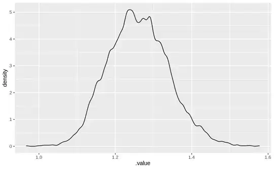
tibble(x=1) %>% add_fitted_draws(hum) %>% ggplot(aes(x = .value)) + geom_density()

is as follows enter image description here The posterior summary is:
                  Estimate Est.Error        Q2.5       Q97.5
b_Intercept       1.468677 0.1037202    1.271352    1.681500
b_hu_Intercept    2.081498 0.1474433    1.802057    2.372279
shape             1.757053 0.3114681    1.203522    2.418776
lp__           -315.947968 1.2657819 -319.090956 -314.508678

I don't see any divergences in the model fit. Also there is pretty good mixing of the chains for the parameters. Given the whole reason for me to consider the hurdle model was to see a model predict zeros in abundance, I am unable to understand the predictions. Shouldn't I see a lot of zeros?

It would be great if someone can throw light on the share a simple test case on using the hurdle model. I am unable to find a nice write up of modeling using hurdle_gamma using brms.

  • Operating System: Ubuntu 18.04
  • brms Version:2.13

2 Answers2

3

Quick note: when including simulation code please always remember to set a seed so that others can reproduce your data.

Shouldn't I see a lot of zeros?

You didn't include a plot, but I will use your code to simulate, run a hurdle model and then make predictions and plot them.

Note I do not use brms so I will simply use two generalised linear models, one to model the zeros and non zeros and one for model the non zeros as a gamma model. This should also help in understanding hurdle models:

set.seed(15)
N <- 1000

non_zero <- rbinom(N, 1, 0.1)
g_vals <- rgamma(n = N, shape = 2, scale = 2)
dat <- data.frame(y = non_zero * g_vals, non_zero, x = 1:N)

Note also that I have renamed your reponse variable to y in accordance with common convention. I am also including x as an index.

So, first we fit a logistic regression to obtain the binomial distribution coefficient, then we fit a gamma glm on the non-zero values to obtain the gamma parameter.

m1 <- glm(non_zero ~ 1, data = dat, family = binomial(link = logit))
m2 <- glm(y ~ 1, data = subset(dat, non_zero == 1), family = Gamma(link = log))

(bin_coef <- plogis(coef(m1)[[1]]))
[1] 0.115

(gamma_coef <- exp(coef(m2)[[1]]))
[1] 4.181137

Here we can note that these are the values we were expecting (0.1 for the binomial and 2*2 = 4 for the gamma.

So now we can make some predictions using these values and plot them:

pred.non_zero <- rbinom(N, 1, bin_coef)
pred.g_vals <- rgamma(n = N, shape = 2, scale = 2)
pred.dat <- data.frame(y = pred.non_zero * pred.g_vals, non_zero = pred.non_zero, x = 1:N)

pred.dat$non_zero <- as.factor(pred.dat$non_zero)
ggplot(pred.dat, aes(x, y, colour = non_zero)) + geom_point()

enter image description here

As expected we do see a lot of zeros.

Robert Long
  • 53,316
  • 10
  • 84
  • 148
  • Hi Robert, thanks for taking the effort to explain based on the glm function. I was looking for a way do it using a bayesian approach using the brms package. Also, I added the image as you have pointed out. – Srivatsa Srinath Jul 19 '20 at 13:51
  • You need to be a little careful because questions about how to use software are off topic here, that's why I answered, making sure to keep it *statistical*. The plot you have included implies that there is either something wrong with the way you fitted the model or the way you made the predictions. – Robert Long Jul 19 '20 at 13:53
  • I understand, thank you, I apologize. I didn't realize it was an issue with my lack of understanding of brms prior to posting the question. – Srivatsa Srinath Jul 19 '20 at 13:59
  • No worries - it seems you've solved it now. I was going to suggest using `predict` - in general that's the way R packages work. – Robert Long Jul 19 '20 at 14:41
3

I had posted the same question in the stan forum and the response was the following: "Try using the predict functions in brms, or analogs. It looks like you’re estimating fitted results, which are conditional averages, not draws from the posterior predictive distribution."

Now when I use (add_predicted_draws instead of add_fitted_draws),

tibble(x=1:100) %>% add_predicted_draws(hum) %>% ggplot(aes(x = .prediction)) + geom_density()

I obtained the following plot

enter image description here

This is the nature of the zero inflation I was expecting from the posterior draws. In was incorrectly looking at conditional averages. Thanks to @franzsf in the stan forum for pointing this out.