2

I would like to know how to model errors introduced by rounding. For example:

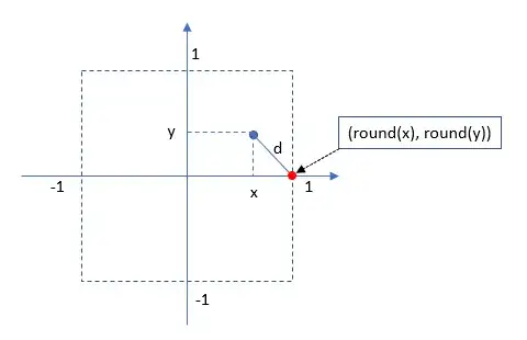
(x,y) and (round(x), round(y))

Suppose that

  • $n$ pairs $(x, y)$ are such as $x$ and $y$ are drawn from a uniform distribution $[-1, 1 [$ and
  • $d$ is given by the Euclidian Distance between $(x, y)$ and respective pair $(round(x), round(y))$.

By histogramming the list of $d$'s results in:

histogram of d

As we can see this distribution is skewed. In my experiments, I checked out the shape of $d$ for 3, 4, 5 variables (see the plots below). I realized that the behavior is always the same:

histograms for xy, xyz, xyzw and xyzwt

My questions are:

  • Why is this distribution skewed?
  • Which distribution should be suitable to model $d$? Is Log-normal the best option?

I understand that Central Limit Theorem is valid for sums of random variables and the Euclidian Distance is not a regular sum. Thus, what should we use to model d?

For clarify, my R script is:

size <- 1000000
x <- runif(size , -1, 1)
y <- runif(size , -1, 1)
z <- runif(size , -1, 1)
w <- runif(size , -1, 1)
t <- runif(size , -1, 1)
x.round <- round(x)
y.round <- round(y)
z.round <- round(z)
w.round <- round(w)
t.round <- round(t)
d.x <- abs(x - x.round)
d.x.y <- sqrt((x - x.round)^2 + (y - y.round)^2)
d.x.y.z <- sqrt((x - x.round)^2 + (y - y.round)^2 + (z - z.round)^2)
d.x.y.z.w <- sqrt((x - x.round)^2 + (y - y.round)^2 + (z - z.round)^2 + (w - w.round)^2)
d.x.y.z.w.t <- sqrt((x - x.round)^2 + (y - y.round)^2 + (z - z.round)^2 + (w - w.round)^2 + (t - t.round)^2)

par(mfrow=c(3,2))
hist(d.x)
hist(d.x.y)
hist(d.x.y.z)
hist(d.x.y.z.w)
hist(d.x.y.z.w.t)
Duloren
  • 143
  • 6
  • 1
    See https://stats.stackexchange.com/a/451376/919 for a closely related discussion. Because of the sharp edge effects, these are nasty distributions to describe mathematically. – whuber Jul 16 '20 at 17:12
  • thank you @whuber . On high order dimension settings, the Euclidean distance is not very useful. – Duloren Jul 18 '20 at 01:08
  • I'm baffled by that remark, for isn't your question about Euclidean distance? – whuber Jul 18 '20 at 16:32

1 Answers1

0

Consider the $x$ and $y$ coordinates separately. In particular, consider the distribution of $|x - \text{round}(x)|$. This will be distributed uniformly on $[0,\frac{1}{2}]$. Whatever rounding point happens to be closest, that distance is between $0$ and $1/2$ and all intermediate points are equally likely. The same argument holds for the y-axis.

Since the coordinates are drawn independently, we can define $\tilde{x}$ and $\tilde{y}$ as independent uniform variables on $[0,\frac{1}{2}]$ and we have:

$\text{distance} = \sqrt{\tilde{x}^2 + \tilde{y}^2}$

Analytically deriving the distribution of this is a bit of a hassle, but consider just the distribution of $\tilde{x}^2$. Squaring a uniform variable does not result in another uniformly distributed variable; in fact this component has a pdf of $x^{-\frac{1}{2}}$ for $x \in [0,\frac{1}{4}]$. The skewness comes from the fact the Euclidean distance is a nonlinear transformation.

Using Mathematica to find the convolution of this variable with itself, and then applying the square-root transformation, yields the following pdf:

$ \begin{cases} \pi & 0<z\leq \frac{1}{4} \\ -2 \left(\csc ^{-1}\left(\frac{2}{\sqrt{4-\frac{1}{z}}}\right)-\csc ^{-1}\left(2 \sqrt{z}\right)\right) & \frac{1}{4}<z<\frac{1}{2} \end{cases} $

which to my knowledge is not any kind of canonical or well-known distribution. Here it is rescaled and superimposed on top of a histogram:

As for the central limit theorem, it actually does apply here despite the nonlinear transformation. Suppose you are working in $d$ dimensions and let $\tilde{x}_i$ be the squared error along the $i$th dimension. As $d \rightarrow \infty$ the mean:

$\frac{1}{d} \sum_{i}^{d} \tilde{x}_i$

will converge to $\frac{1}{12}$ with variance $\frac{1}{180d}$.

We can now apply the univariate delta method with $\theta = \frac{1}{12}$, $\sigma = \frac{1}{180}$, $g(\theta) = \sqrt{\theta}$ and $[g'(\theta)]^2 = \frac{1}{4 \theta}$. The distribution of:

$\sqrt{\frac{1}{d} \tilde{x}_i} = \frac{1}{\sqrt{d}} \sqrt{(x_1 - \text{round}(x_1))^2 + (x_2 - \text{round}(x_2))^2...}$

will be asymptotically normal as $d \rightarrow \infty$ with mean $\frac{1}{2 \sqrt{3}}$ and variance $\frac{d^2}{60}$. Rescaling to remove the $\frac{1}{\sqrt{d}}$, the average rounding error will approach $\frac{\sqrt{d}}{2 \sqrt{3}}$ (meaning it increases with dimension) with a variance approaching $1/60$.

You can kind of see this in the plots you posted, but note that we're taking the limit with respect to dimensions, not sample points. You only went up to $d = 5$.


Note: I deleted a previous answer because I misread a key detail. For some reason I thought you were comparing two different rounded points rather than comparing an unrounded point to the rounded same point.

ZTaylor
  • 16
  • 1