Fixing convergence in SIR model using modified fit-model to fit COVID-19 data

Question

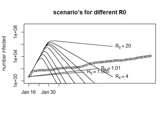
I'm trying to model the data for covid-19 using SIR model in R. I followed the answer of the question, and the blog. I'm using the suggested code, However, the data does not converging. Any suggestion what I'm missing.

# required libraries

library(deSolve)
library(shape)  # for plotting arrows
library(progress)  # for drawing the progress bar



####################################
##
## The basic model (which does not result in the exact solution)
## Adapted from the previous blogpost but with small adaptations
##
####################################

# the data infected represents cumalative sum (cumsum (infected)- (cumsum(recovered)+cumsum(death) )  )  
IpRpD <- c(5,11,26,43,45,45,46,56,56,56,57,57,60,63,63,67,67,75,95,
           97,103,111,118,127,130,137,149,158,159,152,152,159,168,
           171,188,194,216,237,261,335,385,456,561,637,743,798,869,
           1020,1091,1148,1176,1196,1296,1395,1465,1603,1619,1657,1792,
           1887,1986,2217,2249,2254,2241,2327,2459,2745,2883,3169,3291,
           3732,4028,4142,4695,4952,5901,6314,7101,7683,8436,9124,9852,
           10645,11234,11962,12559)
# only recovered not cummalative sum
R <- c(310,320,204,342,246,250,203,189,188,162,194,178,107,156,85,162,187,85,171,73,101,63,150,
       213,164,206,150,43,115,55,31,45,62,25,22,33,19,30,26,8,9,10,12,0,6,2,4,6,11,1,1,7,1,5,3,
       7,8,6,4,9,0,3,5,4,3,3,0,3,2,2,0,0,3,0,1,0,0,0,1,0,0,0,0,0,0,0,0,0,0)

# Only death NOT cuumalative
D <- c(9,5,3,3,6,5,11,8,6,7,10,7,9,2,3,2,2,0,2,5,3,4,2,1,1,2,1,4,1,1,2,2,2,1,1,2,0,0,1,1,0,0,0,0,
       0,0,0,0,1,0,0,0,0,0,0,0,0,0,0,0,0,0,0,0,0,0,0,0,0,0,0,0,0,0,0,0,0,0,0,0,0,0,0,0,0,0,0,0,0)



Infected <-IpRpD
Day <- 1:(length(Infected))
N <- 4921638 #population

# ODE equation used for fitting
#
# I have removed the R(t) in comparison 
# to the function used in the odler blogpost
# because we are not gonna use that value
# also we have anyway: R(t) = N(0) - N(t) - I(t)
SIR <- function(time, state, parameters) {
  par <- as.list(c(state, parameters))
  with(par, {
    dS <- -beta/N * I * S
    dI <- beta/N * I * S - gamma * I
    list(c(dS, dI))
  })
}

#
# cost function to be optimized in the fitting
#
RSS <- function(parameters) {
  names(parameters) <- c("beta", "gamma")
  out <- ode(y = init, times = Day, func = SIR, parms = parameters)
  fitInfected <- out[,3]
  # fitInfected <- N-out[,2] # this would be a better comparison since the data is not the number of Infectious people
  sum((Infected - fitInfected)^2)
}

# starting condition
init <- c(S = N-Infected[1], I = Infected[1])
# init <- c(S = N-Infected[1], I = Infected[1]-R[1]-D[1])  use this starting condition when applying the different line in the RSS function

# performing the fit
Opt <- optim(c(0.5, 0.5), RSS, method = "L-BFGS-B", lower = c(0, 0), upper = c(1, 1)) # optimize with some sensible conditions
Opt$message


Opt_par <- setNames(Opt$par, c("beta", "gamma"))
Opt_par
##     beta     gamma 

# plotting the result
t <- 1:120 # time in days
fit <- data.frame(ode(y = init, times = t, func = SIR, parms = Opt_par))

plot(Day,Infected, xlim = range(Day), ylim = range(Infected) )
lines(t,fit[,3])

###########################
##
## Alternative model which provides a better fit
##
############################

# We transform the equations and instead of 
# parameters beta and gamma
# we use parameters 
#
#    K = beta-gamma
#    R0 = beta/gamma
#
#    or    
#
#    beta =   K * R0/(R0-1)  
#    gamma =  K *  1/(R0-1)
#  
# then the equations become
#
# dS  = I * K * (-S/N *  R0)/(R0-1)
# dI  = I * K * ( S/N *  R0 - 1)/(R0-1)  
# note in the beginning, S/N = 1
# then in the start you get this approximate exponential growth
# dI = I * K * (1)


SIR2 <- function(time, state, parameters) {
  par <- as.list(c(state, parameters))
  with(par, {
    dS <- I * K * (-S/N *  R0/(R0-1))
    dI <- I * K * ( S/N *  R0/(R0-1) - 1/(R0-1))  
    list(c(dS, dI))
  })
}

RSS2 <- function(parameters) {
  names(parameters) <- c("K", "R0")
  out <- ode(y = init, times = Day, func = SIR2, parms = parameters)
  fitInfected <- out[,3]
  #fitInfected <- N-out[,2]
  sum((Infected - fitInfected)^2)
}

### Two functions RSS to do the optimization in a nested way
###
### This nesting requires a lot more computational power
### However, it makes that we have to worry less about the different scale 
### of the parameters

Infected_MC <- Infected
SIRMC2 <- function(R0,K) {
  parameters <- c(K=K, R0=R0)
  out <- ode(y = init, times = Day, func = SIR2, parms = parameters)
  fitInfected <- out[,3]
  #fitInfected <- N-out[,2]
  RSS <- sum((Infected_MC - fitInfected)^2)
  return(RSS)  
}
SIRMC <- function(K) {
  optimize(SIRMC2, lower=1,upper=10^5,K=K, tol = .Machine$double.eps)$objective
}

# wrapper to optimize and return estimated values
getOptim <- function() {
  opt1 <- optimize(SIRMC,lower=0,upper=1, tol = .Machine$double.eps)
  opt2 <- optimize(SIRMC2, lower=1,upper=10^5,K=opt1$minimum, tol = .Machine$double.eps)
  return(list(RSS=opt2$objective,K=opt1$minimum,R0=opt2$minimum))
}

# starting condition
#init <- c(S = N-Infected[1], I = Infected[1]-R[1]-D[1])
init <- c(S = N-Infected[1], I = Infected[1])

# performing the fit 
# starting K=0.3, R0 = 2
Opt2 <- optim(c(0.3, 2), RSS2, method = "L-BFGS-B", 
              hessian = TRUE, control = list(parscale = c(10^0,10^0), factr = 1)) 
Opt2

Opt3 <- getOptim()
Opt3

Opt_par2 <- setNames(Opt2$par, c("K", "R0"))
Opt_par3 <- setNames(Opt3[2:3], c("K", "R0"))


# plotting the result
t <- seq(1,120,1) # time in days
fit1 <- data.frame(ode(y = init, times = t, func = SIR , parms = Opt_par))
fit2 <- data.frame(ode(y = init, times = t, func = SIR2, parms = Opt_par2))
fit3 <- data.frame(ode(y = init, times = t, func = SIR2, parms = Opt_par3))

plot(Day,Infected, xlim = range(Day), ylim = range(Infected), 
          log = "", xaxt = "n",
     main = "Infected(including Recovered and Death)", xlab = "Day", ylab = "number infected")
lines(t, fit3[,3], col = 1)
lines(t, fit2[,3], col = 4, lty = 2)
lines(t, fit1[,3], col = 2, lty = 3)
axis(1, at = 1:90, labels = rep("",90), tck = -0.01)
# these labels are not valid for the current date 
axis(1, at = c(1,8,15,22), labels = c("Jan 16", "Jan 23", "Jan 30", "Feb 6"))  

text(t[183]+2,fit1[183,3]+1800,"old optim fit",pos=4, col=2)
text(t[183]+2,fit1[183,3],expression(R[0] == 2.07),pos=4, col=2)
text(t[183]+2,fit1[183,3]-1400,expression(RSS == 74.3 %*% 10^6),pos=4, col=2)

text(t[220]+3,fit2[220,3]+3200,"new optim fit",pos=3, col=4)
text(t[220]+3,fit2[220,3]+1400,expression(R[0] == 1.0054626),pos=3, col=4)
text(t[220]+3,fit2[220,3],expression(RSS == 6.5 %*% 10^6),pos=3, col=4)

text(t[240]-3,fit3[240,3],"nested algorithm",pos=1, col=1)
text(t[240]-3,fit3[240,3]+700-2500,expression(R[0] == 1.005332),pos=1, col=1)
text(t[240]-3,fit3[240,3]-700-2500,expression(RSS == 5.9 %*% 10^6),pos=1, col=1)

x1 <- t[240]-3;    x2 <- t[225];
y1 <- fit3[240,3]; y2 <- fit3[225,3]
Arrows(x1,y1,x1+(x2-x1)*0.65,y1+(y2-y1)*0.65, col = 1)

x1 <- t[220]+2;    x2 <- t[227];
y1 <- fit2[220,3]; y2 <- fit2[227,3]
Arrows(x1,y1,x1+(x2-x1)*0.6,y1+(y2-y1)*0.6, col = 4)

x1 <- t[183]+2;    x2 <- t[183];
y1 <- fit1[183,3]; y2 <- fit1[183,3]
Arrows(x1,y1,x1+(x2-x1)*0.6,y1+(y2-y1)*0.6, col = 2)




####################
##
## Graph with various values of R0
##
#######################

# starting condition
#init <- c(S = N-Infected[1], I = Infected[1]-R[1]-D[1])
init <- c(S = N-Infected[1], I = Infected[1])

Infected_MC <- Infected
SIRMC3 <- function(R0,K) {
  parameters <- c(K=K, R0=R0)
  out <- ode(y = init, times = Day, func = SIR2, parms = parameters)
  fitInfected <- out[,3]
  #fitInfected <- N-out[,2]
  RSS <- sum((Infected_MC - fitInfected)^2)
  return(RSS)  
}

plot(Day,Infected, xlim = range(Day), ylim = c(1,10^9), 
     log = "y", xaxt = "n",
     main = "scenario's for different R0", xlab = "", ylab = "number infected")

axis(1, at = 1:30, labels = rep("",30), tck = -0.01)
axis(1, at = c(1,8,15,22), labels = c("Jan 16", "Jan 23", "Jan 30", "Feb 6"))


for (i in 1:10) {
  R0 <- c(1.005,1.01,1.05,1.1,1.2,1.5,2,2.5,4,20)[i]
  K <- optimize(SIRMC3, lower=0,upper=1,R0=R0, tol = .Machine$double.eps)$minimum
  parameters <- c(K,R0)
  xd <- seq(1,60,0.01)
  if (i == 1) {
    xd <- seq(1,40,0.01)
  }
  if (i == 2) {
    xd <- seq(1,50,0.01)
  }
  out <- ode(y = init, times = xd, func = SIR2, parms = parameters)
  lines(xd,out[,3])
  text(tail(xd,1),tail(out[,3],1),bquote(R[0] == .(R0)), pos =4)
}

Answer 1

The problem is that search for the optimal $K$ for a given $R_0$ is ending up in a local optimum.

Ks <- seq(0,1,0.001)
plot(Ks,Vectorize(SIRMC2)(1.1,Ks), type = "l",
     xlab = "K", ylab = "RSS", 
     main = "RSS as function of K for fixed R0 = 1.1")

You get the value $K=1$ on the right instead the value around 0.07. I am not sure whether there are simple functions in R that can solve this automatically and easily. My way to improve the code would be to do an initial grid search and improve with an optimizer. (or since you know that the curve is intitally exponential you could use that as starting value).