Can I use the early response to a treatment to predict the full effect? - Dealing with regression towards the mean

Question

Suppose I have a 6 week weight-loss program, that I know is only effective in a fraction of the population. I weight the participants at baseline, after 1 week and after the full 6 weeks.

$$ T_0 = Baseline $$ $$ T_1 = 1\ Week $$ $$ T_2 = 6\ Weeks $$

I want to investigate if the effect at after 1 week can indicate if it is worthwhile to continue the program.

A naive approach would be to see if $$ WLoss_{T1} = \frac{W_{T0} - W_{T1}}{W_{T0}} $$ is correlated with $$ WLoss_{T2} = \frac{W_{T1} - W_{T2}}{W_{T1}}$$

and maybe decide some minimal meaningful weight loss (eg $WLoss_{T2} > 2 \%$) and use a receiver operating characteristic (ROC) analysis to see how well $WLoss_{T1}$ can predict this weight loss.

This would, however, underestimate the correlation between $WLoss_{T1}$ and $WLoss_{T2}$ due to the mathematical coupling between $WLoss_{T1}$ and $WLoss_{T2}$ (both use $W_{T1}$). A persons weight loss after 1 week could simply be due to measurement error and random variation in body weight (random error), and the next measurement would likely be closer to baseline, due to the same random variation in body weight measurement, giving a negative correlation between $WLoss_{T1}$ and $WLoss_{T2}$.

The problem can also be viewed as regression towards the mean.

What are appropriate ways of avoiding the bias caused by this mathematical coupling?

Answer 1

Followig comments below rolando2 post, I was about to suggest you to make the regression: $$Weight_{i,t} = c_i + \alpha . 1(T_1) + \gamma . 1(T_2) + \epsilon_{i,t}$$ Then you would get a matrix of variance-covariace of the coefficients. Maybe it would be enough to look at $cov(\alpha,\beta)$ (and to check somehow that it is significantly positive). But, if I make no mistake, you would have in fact the same problem as described in the question.

Otherwise, if you have a lot of observations, you might divide you sample into cells c (with lots of people; for instance by age-gender). Make on each cell the following regression: $$log(Weight_{i \in c,t}) = c_i + \alpha_c . 1(T_1) + \gamma_c . 1(T_2) + \epsilon_{i,t}$$ In each cell c, there is no reason why the mean effect of $T_1$ and the mean effect of $T_2$ would be subject to individual measurement error.

Then you regress: $\gamma_c = \delta . \gamma_c + \zeta_{i,t}$.

You are interested in $\delta$. Please note that significancy of $\delta$ will be underestimated...because the dependent variable is itself estimated (and the explanatory variable). I would say this does not require to be dealt with if you have enough people in each cell so that the first steps estimations are precise enough. If you do not have many people, there are formula to de-bias the variance when the dependent variable is estimated - but this might be more difficult here as both the dependent variable and the explanatory variable are estimated.

Answer 2

You seem to be talking about an intervention working. If it is only worth persisting with the intervention, if the intervention works, then how do we tell whether it works? This leads to the counter-factual of "What would have happened, had the person not received the intvention?" Otherwise, you might just attribute random fluctuation and regression to the mean to the intervention

To tell what would have happened, if a person had not taken an intervention, you would need a pretty reliable prediction model for what happens without intervention including the uncertainty around that. E.g. such a model might give you the (correlated) prediction for your two time points and you can check whether the change is larger than what you expect for most patients without intervention.

Difficulities include that you would need a pretty large dataset representative of the relevant target population to build a good model (alternatively, you could replace a model with elicited expert opinions about trajectories without intervention, but that is also not very easy). Additionally, it may be that for an individual it might often be quite hard to tell the difference between chance variation and a large causal effect (depends, also depends a lot on the time scale and the size of the intervention effect).

Answer 3

I have the feeling you are over-complicating things: differences...correlation...ROC. You have longitudinal data collected at 3 time points; you could take advantage of this to create a single model, a random-effects model (mixed model; longitudinal model). I think it would take into account everything you have mentioned and would do so in, as John Willett likes to say, one swell foop.

Answer 4

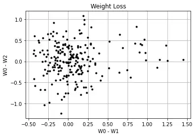
If I understand you correctly, you want to know whether you can reliably classify your participants based on their early weight loss. So it's basically a question of classification. I recon you also have a training data set, with measurements $W0$, $W1$, and $W2$. Let's assume your data look like this:

or, relative to the baseline:

You could, as you suggested, declare some arbitrary boundary (0.02) for the effective weight loss and label your data accordingly:

The simplest thing to do now, if you just want to know whether the early weight loss is indicative for the later weight loss, would be to run a t-test on the x-axis (the early weight loss) of the two groups. In Python:

import numpy as np
import matplotlib.pyplot as plt

mu0     =  90
sigma0  =  15
sigma1  =    .2
sigma2  =   1
Na      =  20
Nb      = 200
effect1 =    .99
effect2 =    .975

rng = np.random.RandomState(42)
w0 = rng.normal(mu0, sigma0, Na+Nb)
w1 = np.concatenate([
  (effect1 * w0)[:Na ] + rng.normal(0, sigma1, Na),
  (          w0)[ Na:] + rng.normal(0, sigma1, Nb)
])
w2 = np.concatenate([
  (effect2 * w0)[:Na ] + rng.normal(0, sigma2, Na),
  (          w0)[ Na:] + rng.normal(0, sigma2, Nb)
])

r1 = (w0-w1)/w0
r2 = (w0-w2)/w0

# t-test on the x-axis
from scipy import stats
tt = stats.ttest_ind(r1[r2<.02], r1[r2>.02])
print(tt)

produces:

Ttest_indResult(statistic=-11.912202742445448, pvalue=1.581946945815335e-25)

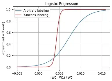
But you probably want to have a classification algorithm, so you'll need to train a model. A logistic regression will give you not only the probabilities of class membership, but also the p-values for the coefficients, thus answering your initial question:

# logistic regression
import statsmodels.api as sm
logit_model=sm.Logit(r2>.02, sm.add_constant(r1))
result=logit_model.fit()
print(result.summary())

gives you:

                           Logit Regression Results                           
==============================================================================
Dep. Variable:                      y   No. Observations:                  220
Model:                          Logit   Df Residuals:                      218
Method:                           MLE   Df Model:                            1
Date:                Tue, 05 May 2020   Pseudo R-squ.:                  0.4436
Time:                        21:25:18   Log-Likelihood:                -42.182
converged:                       True   LL-Null:                       -75.814
Covariance Type:            nonrobust   LLR p-value:                 2.373e-16
==============================================================================
                 coef    std err          z      P>|z|      [0.025      0.975]
------------------------------------------------------------------------------
const         -3.4028      0.405     -8.393      0.000      -4.197      -2.608
x1           472.5083     77.561      6.092      0.000     320.491     624.526
==============================================================================

If you want to make it less arbitrary and more sophisticated, you can, instead of arbitrary labeling, use clustering (e.g. K-means) on the two-dimensional data and use cluster labels for training your classifier:

from sklearn.cluster import KMeans
# important: need to scale the axes appropriately!
X_SCALE = (np.max(r2) - np.min(r2)) / (np.max(r1) - np.min(r1))
w = np.concatenate([X_SCALE*r1.reshape([-1, 1]), r2.reshape([-1, 1])], axis=1)
k2 = KMeans(n_clusters=2).fit(w)
fig, ax = plt.subplots()
ax.plot(r1[k2.labels_==0], r2[k2.labels_==0], '.', c='orangered')
ax.plot(r1[k2.labels_==1], r2[k2.labels_==1], '.', c='green')
ax.set(xlabel='(W0 - W1) / W0', ylabel='(W0 - W2) / W0', title='Relative Weight Loss, Clustered')
ax.grid()
ax.legend(["Not working", "Working"])
plt.show()

Logistic regression on data labeled this way is slightly different:

                           Logit Regression Results                           
==============================================================================
Dep. Variable:                      y   No. Observations:                  220
Model:                          Logit   Df Residuals:                      218
Method:                           MLE   Df Model:                            1
Date:                Tue, 05 May 2020   Pseudo R-squ.:                  0.8536
Time:                        21:30:47   Log-Likelihood:                -10.787
converged:                       True   LL-Null:                       -73.691
Covariance Type:            nonrobust   LLR p-value:                 3.389e-29
==============================================================================
                 coef    std err          z      P>|z|      [0.025      0.975]
------------------------------------------------------------------------------
const         -7.7915      2.166     -3.597      0.000     -12.037      -3.546
x1          1732.4376    614.892      2.817      0.005     527.271    2937.604
==============================================================================

The following graph shows the logistic regression for arbitrary (manual cutoff) labeling and for K-means labeling:

Update:

Spurious correlation ("mathematical coupling") is not an issue here. Observe a set where the long-term weight loss is not related to the early weight loss:

rng = np.random.RandomState(42)
w0 = rng.normal(mu0, sigma0, Na+Nb)
w1 = np.concatenate([
  (effect1 * w0)[:Na ] + rng.normal(0, sigma1, Na),
  (          w0)[ Na:] + rng.normal(0, sigma1, Nb)
])
w2 = w0 + rng.normal(0, 2*sigma1, Na+Nb)

You can define a "meaningful" weight loss to be as low as 0.5%, but it will be equally distributed over the two groups, with and without early weight loss:

The mean relative early weight losses won't differ between the groups:

stats.ttest_ind(r1[r2<.005], r1[r2>.005])

Ttest_indResult(statistic=-0.17757452954060468, pvalue=0.8592220151288611)

and you'll get the same p-value in logistic regression.

If you do K-means, it will find two clusters, but along the x-axis (early weight loss). You need to check that the long-term losses differ in the two clusters.