6

glm() of the following data gives intercept 0.56916 and slope x .018. But the true slope should be 1/10. Does anybody know why glm() can not recover the true slope? Thanks.

R> tmp = data.frame(x=seq_len(100), y=rpois(100, lambda=seq_len(100)/10))
R> fit = glm(y ~ x, family=poisson, data=tmp)
R> fit

Call:  glm(formula = y ~ x, family = poisson, data = tmp)

Coefficients:
(Intercept)            x  
    0.56916      0.01812  

Degrees of Freedom: 99 Total (i.e. Null);  98 Residual
Null Deviance:      252.6 
Residual Deviance: 125.1    AIC: 442.3
R> library(ggplot2)
R> p=qplot(tmp$x, predict(fit))
R> ggsave(p, file='/tmp/glm_poisson_fit.png')
Saving 7 x 7 in image
R> 
user1424739
  • 424
  • 2
  • 9
  • 3
    1. Your sample is too small. 2. Poisson-GLM uses log-link by default. – Michael M Apr 13 '20 at 05:33
  • Try the identity link (you might need to supply start values). – Glen_b Apr 13 '20 at 06:37
  • @meriops this comment is confusing. Neither the example assume “different means”, nor GLM estimates “single mean”. In both cases we are talking about conditional mean being a function of X. – Tim Apr 13 '20 at 09:14

1 Answers1

12

Poisson regression model is

$$ \log (\operatorname{E}(Y\mid\mathbf{x}))=\alpha + \mathbf{\beta}' \mathbf{x} $$

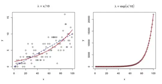
So you are fitting different function to your data, then the one that generated it, so it would have different parameters. Poisson regression uses by default the log as a link function. For your simulation to be in-line with the Poisson regression model, you would need to draw samples from

$$ Y \sim \mathcal{P}(\,\exp[\alpha + \mathbf{\beta}'\mathbf{x} ]\,) $$

Translating this into R code, that gives:

set.seed(123)
n <- 100

x <- seq_len(n)
y <- rpois(n, x/10)
beta <- glm(y ~ x, family='poisson')$coef
plot(x, y)
curve(x/10, min(x), max(x), col='blue', lty=2, lwd=2, add=TRUE)
curve(exp(beta[1] + beta[2] * x), min(x), max(x), col='red', lwd=2, add=TRUE)
title(expression(lambda == x/10))

x <- seq_len(n)
y <- rpois(n, exp(x/10))
beta <- glm(y ~ x, family='poisson')$coef
plot(x, y)
curve(exp(x/10), min(x), max(x), col='blue', lty=2, lwd=2, add=TRUE)
curve(exp(beta[1] + beta[2] * x), min(x), max(x), col='red', lwd=2, add=TRUE)
title(expression(lambda == exp(x/10)))

enter image description here

As you can see on the plots, the true regression line (blue dashed line) in first case differs from the regression line (red line) predicted by the model, while in second case they match so closely, that they are indistinguishable on the plot.

Tim
  • 108,699
  • 20
  • 212
  • 390