(This question is a bit related to a previous question of mine, but that question was about between subject comparison while this question is specifically about making inferences the group mean.)
When analyzing data using a hierarchical Bayesian model you sometimes don't want to make inferences on the individual subjects but rather on the group level (e.g. for girls aged 10 the most credible test score is 100 with a 95% credible interval of [75, 125]). When building such a model using an MCMC framework, for example JAGS/BUGS, I see two ways of getting at the group level mean. Either I can use the mean of the prior ($\mu_\text{gr}$ in the diagram below.) on the mean of the sampling distribution or, for each iteration of the MCMC algorithm I can calculate the mean of all the subject means (that is the mean of all $\mu_\text{subj}$ in the diagram below). If I want to make inferences about the group mean which of these two alternatives should I use?
As a test to see what happens when using the the two different alternatives I ran a model with simulated data.
Here is a Kruschke style diagram of a hierarchical model where we estimate the mean $\mu_\text{subj}$ for a number of subjects with a normally distributed group prior on $\mu_\text{subj}$ with mean $\mu_\text{gr}$.

Here is JAGS and R code for specifying the model above and simulating data for 50 subjects where each subject gets a mean that is randomly normally distributed with $\mu=0$ and $\sigma=1$. The JAGS model is then run for 5000 iterations and each iteration the mean of the prior, group_mu, and the calculated mean of the subjects, mean_mu <- mean(mu[]), is saved.
library(rjags)
model_string <- "model {
  for(i in 1:length(y)) {
    y[i] ~ dnorm( mu[subject[i]], precision[subject[i]])
  }

  mean_mu <- mean(mu[])
  for(subject_i in 1:n_subject) {
    mu[subject_i] ~ dnorm(group_mu, group_precision)
    precision[subject_i] <- 1/pow(sigma[subject_i], 2)
    sigma[subject_i] ~ dunif(0, 10)
  }

  group_mu ~ dunif(-10, 10)
  group_precision <- 1/pow(group_sd, 2)
  group_sd ~ dunif(0, 10)
}"

# Creating fake data
n <- 10
n_subject <- 50
subject_mean <- rnorm(n_subject, mean=0, sd=1)
y <- rnorm(n * n_subject, mean=rep(subject_mean, each=n), sd=1)
subject <- rep(1:n_subject, each=n)

# Running the model with JAGS
jags_model <- jags.model(textConnection(model_string),
                         data=list(y=y, subject=subject, n_subject=n_subject),
                         n.chains= 3, n.adapt= 1000)
update(jags_model, 1000)
jags_samples <- jags.samples(jags_model,
                             variable.names=c("group_mu", "mean_mu"),
                             n.iter=5000)
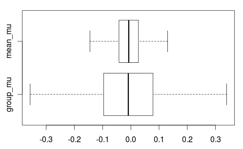
Looking at quantiles and boxplots of mean_mu and group_mu show that they are both centered around the true group mean but they differ a lot in spread with the 95% credible interval being much wider for group_mu than for mean_mu.
quantile(jags_samples$mean_mu, c(0.025, 0.5, 0.975))
##       2.5%         50%       97.5%
##  -0.10804263 -0.00741235  0.09216414
quantile(jags_samples$group_mu, c(0.025, 0.5, 0.975))
##        2.5%          50%        97.5%
##  -0.262734656 -0.008996673  0.248624938
boxplot(jags_samples, outline=F, horizontal=T)
So if I want to make inferences about the group mean which distribution should I use, group_mu or mean_mu? For me this is not clear and any explanation why one is to be preferred over the other is highly appreciated!