1

Trying to understand the role eigenvalues and vectors play in least squares solutions

Reading answers to this post, Relation between best fit line and eigenvector of maximum eigen value of an estimated covariance matrix

It appears that eigenvectors actually point in the direction of the regression line. Is this correct?

Lets say I have a problem with 2 independent variables and 1 dependent variable.

I collect data for each X1 and X2 and corresponding Y

I want to make a plane that fits this data, so that I could input any X1 and X2 and get an approximate solution for Y

This would be the method I use http://www.real-statistics.com/multiple-regression/least-squares-method-multiple-regression/ (I haven't tried to implement it yet)

What do the eigenvectors and values represent in this case?

mckenneth
  • 11
  • 1
  • 1
    The regression line will not coincide with any eigenvector except in special cases. This phenomenon is known as "regression to the mean." As far as the rest of your question goes, there are two different sets of eigensystems, both of which are natural and useful: the eigensystem of the matrix created by the columns of the regressors and the eigensystem of that matrix augmented by the response $Y.$ Which one are you asking about? – whuber Sep 05 '19 at 15:49

2 Answers2

1

I have taken a very simple example to explain the relationship of eigen vectors/ principal components w.r.t linear regression

    # The formula is y=2x1 + 5
    import numpy as np
    import random
    x1=np.random.randint(50,size=50)
    y1=[2*x1[i] + np.random.randint(30) for i in list(range(50))]

enter image description here

Now we will fit the linear regression

    from sklearn.linear_model import LinearRegression
    reg = LinearRegression().fit(x1.reshape(-1,1), y1)
    plt.figure()
    plt.scatter(x1,y1)
    plt.plot(x1,[reg.coef_[0]*x + reg.intercept_ for x in x1],color='red')
    plt.show()

enter image description here

Now what we want to do is find out the vector that best finds the direction of maximum variance. This is indirectly the regression line

    %matplotlib inline
    import matplotlib.pyplot as plt
    import seaborn as sns; sns.set()
    from sklearn.decomposition import PCA
    pca = PCA(n_components=2)
    X=np.array(list(zip(x1,y1)))
    pca.fit(X)

    def plot_vector_extensions(v0, v1,color):
        plt.arrow(v0[0], v0[2], v1[0]-v0[0], v1[2]-v0[2],color=color)
        plt.scatter(v0[0],v0[2],color='yellow')
        plt.scatter(v1[0],v1[2],color='yellow')

    # Plot the data
    plt.scatter(X[:, 0], X[:, 1], alpha=0.2,color='blue')
    # Plot the first component
    v = pca.components_[0] * np.sqrt(pca.explained_variance_[0])
    plot_vector_extensions(pca.mean_, pca.mean_ + v,color='red')
    # Plot the first component
    v = pca.components_[2] * np.sqrt(pca.explained_variance_[2])
    plot_vector_extensions(pca.mean_, pca.mean_ + v,color='black')
    plt.show()

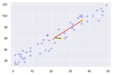
enter image description here

We can see that the first principal component ( marked in red ) in a way depicts the line close to the regression line.

I hope this helps you understand the relationship

Anant Gupta
  • 300
  • 1
  • 3
  • 1
    I would like to suggest that an example with a *low* absolute correlation would be more informative because it would show how the linear regression differs from any eigendirection. This example may leave readers with the false impression that an eigendirection may be "close to the regression line." – whuber Sep 05 '19 at 15:47
1

I was curious about the relationship between eigenvalues/vectors and least squares regression as well. I made widget in Sage (free math software based on python) to explore the question. The code is at the bottom of this post.

Below is a screenshot of the widget. The purple line is the regression line, the blue lines are the eigenvectors multiplied by their eigenvalues. The data points are normalized (subtracted mean, divided by standard deviation).

From the screenshot or from playing around with the values, it's clear that the eigenvectors in most cases don't point in the same direction as the regression line.
Purple least squares line, blue eigenvectors


However, there is a connection between the eigenvalues and the regression line (when the data is standardized): the largest eigenvalue is equal to 1 + the regression coefficient, but this relationship goes away when the data is not normalized.

Perhaps someone else can explain exactly why that is :-)


You should be able to copy-paste this into the Sage notebook to make it work. Or run it online on cocalc.com.

import numpy as np
from numpy import linalg as LA

@interact
def f(gauss_sigma=slider(0.01,50,step_size=0.5, default=0.2), 
      slope=slider(-5,5,step_size=0.1, default=0.2),
      points=slider(10,200,step_size=10, default=20),
      seed=slider(10,20,step_size=1, default=10)):

l = points
sigma = gauss_sigma

T = RealDistribution('gaussian', sigma, seed = seed)
ranvals = [T.get_random_element() for i in range(l)]

xpts = list(range(l))
ypts = [slope*i+ranvals[i] for i in range(l)]

#Means
y_mean = mean(ypts)
x_mean = mean(xpts)
#Subtract means
xpts = [i-x_mean for i in xpts]
ypts = [i-y_mean for i in ypts]
#New means(=(0,0))
y_mean = mean(ypts)
x_mean = mean(xpts)
ympt = point((0, y_mean), color="red")
xmpt = point((x_mean, 0), color="red")
#Divide by standard deviation
xstd = std(xpts).n()
ystd = std(ypts).n()

xpts = [i/xstd for i in xpts]
ypts = [i/ystd for i in ypts]

pts = [[xpts[i], ypts[i]] for i in range(l)]

s = scatter_plot(pts)

#Covariance matrix
covma = np.cov(xpts,ypts)
corma = np.corrcoef(xpts,ypts)

#Eigenvalues, eigenvectors
w, v = LA.eig(covma)
eig1 = w[0]*vector(v[:,0])
eig2 = w[1]*vector(v[:,1])

eig1line = line([(x_mean,y_mean),(eig1[0]+x_mean, eig1[1]+y_mean)], zorder=10)
eig2line = line([(x_mean,y_mean),(eig2[0]+x_mean, eig2[1]+y_mean)], zorder=11)

#Regression line, OLS
var('x,b,d')
model(x) = b*x + d
regr = find_fit(pts, model)
f(x) = regr[0]*x + regr[1]
regr_line = line([(-35, f(-35).rhs()) ,(35,f(35).rhs() )], color="purple")

#Ellipses
from math import acos
ang = acos(vector(v[:,0]).dot_product(vector([1,0])))
elip = ellipse((x_mean,y_mean), w[0]*vector(v[:,0]).norm(), w[1]*vector(v[:,1]).norm(), ang, color="grey")

show(s + ympt + xmpt + eig1line + eig2line + regr_line, #+ elip,
     xmin=-5, xmax=5, ymin=-5, ymax=5, aspect_ratio=1, figsize=10)

print("Covariance matrix:", covma, "\n",
      "Correlation matrix.", corma, "\n",
      "Eigenvalues:",w,
      "Eigenvectors:", v, "\n",
      "Regr coeffs:", regr, "\n",
      sep="\n")
john.abraham
  • 141
  • 4