Testing anova hypothesis with contrasts in R and SPSS

Question

Using data and answers from this question I was trying to test the hypothesis $H_0:-3\mu_1-\mu_2+\mu_3+3\mu_4=0$

set.seed(42)
sample.data <- data.frame(IV=factor(rep(1:4, each=20)),
                          DV=rep(c(-3, -1, 1, 3), each=20) + rnorm(80))
library(car)
Anova(lm(DV ~ C(IV, c(-3, -1, 1, 3), 1), data=sample.data), type="III")

Anova Table (Type III tests)

Response: DV
                          Sum Sq Df  F value Pr(>F)    
(Intercept)                 0.03  1   0.0278 0.8681    
C(IV, c(-3, -1, 1, 3), 1) 407.08  1 347.9506 <2e-16 ***
Residuals                  91.25 78                    
---
Signif. codes:  0 ‘***’ 0.001 ‘**’ 0.01 ‘*’ 0.05 ‘.’ 0.1 ‘ ’ 1

But when I tried to verify my result with SPSS i got

SPSS results

So my question is why $F$ statistics are different? My guess is that I might have misspecified contrasts in R. I as well tried to set type="II", but as this is balanced sample the $F$'s are the same.

I also have an additional question, concerning $F$'s value of (Intercept) term in the output of R, is this a statistic for testing whether the intercept in the model is zero?

Nice question. But please run `set.seed(1234)` (or a seed of your choice) before creating the sample data to make the results reproducible. Thanks. — Aaron left Stack Overflow, Oct 22 '12 at 14:32

score 3 · Accepted Answer · edited Nov 26 '14 at 16:37

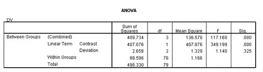
The SPSS model has four terms in it (intercept plus a linear contrast term plus two deviation terms). The R model only has two (intercept plus linear contrast). This means the residual term in SPSS is both smaller and has less df than the model in R. Note that 88.596 + 2.658 = 91.25, so the two models have the same total sum of squares but are dividing it up differently.

To get the same output as SPSS, add any two contrasts that aren't linear and that result in the full basis for the four terms.

Here are quadratic and cubic contrasts:

> c1 <- c(-3, -1, 1, 3)
> c23 <- cbind(c(4, 1, 1, 4), c(-8, -1, 1, 8))
> m <- lm(DV ~ C(IV, c1, 1) + C(IV, c23, 2), data=sample.data)
> anova(m)
# Analysis of Variance Table

# Response: DV
#               Df Sum Sq Mean Sq  F value Pr(>F)    
# C(IV, c1, 1)   1 407.08  407.08 349.1991 <2e-16 ***
# C(IV, c23, 2)  2   2.66    1.33   1.1399 0.3252    
# Residuals     76  88.60    1.17

Here are dummy variables on the first and fourth levels.

> cxx <- cbind(c(1, 0, 0, 0), c(0, 0, 0, 1))
> m <- lm(DV ~ C(IV, c1, 1) + C(IV, cxx, 2), data=sample.data)
> anova(m)
# Analysis of Variance Table
# 
# Response: DV
#               Df Sum Sq Mean Sq  F value Pr(>F)    
# C(IV, c1, 1)   1 407.08  407.08 349.1991 <2e-16 ***
# C(IV, cxx, 2)  2   2.66    1.33   1.1399 0.3252    
# Residuals     76  88.60    1.17

To get the same output for just the linear term, it's perhaps easier to treat IV as continuous and just add the polynomial terms.

> sample.data$IVn <- as.numeric(sample.data$IV)
> m <- lm(DV ~ IVn + I(IVn^2) + I(IVn^3), data=sample.data)
> anova(m)
# Analysis of Variance Table
# 
# Response: DV
#           Df Sum Sq Mean Sq  F value Pr(>F)    
# IVn        1 407.08  407.08 349.1991 <2e-16 ***
# I(IVn^2)   1   1.95    1.95   1.6723 0.1999    
# I(IVn^3)   1   0.71    0.71   0.6075 0.4381    
# Residuals 76  88.60    1.17

You could also fit it with polynomial contrasts, but I don't think it's easy to get the linear term only in an ANOVA table, but you could get the coefficients. Notice that 18.687^2 = 349.2, so it's the same result as before, just presented differently.

> m <- lm(DV ~ C(IV, "contr.poly"), data=sample.data)
> summary(m)
# 
# Call:
# lm(formula = DV ~ C(IV, "contr.poly"), data = sample.data)
#
# Residuals:
#     Min      1Q  Median      3Q     Max 
# -2.9922 -0.5409  0.1351  0.6918  2.1662 
#
# Coefficients:
#                       Estimate Std. Error t value Pr(>|t|)    
# (Intercept)            0.02015    0.12071   0.167    0.868    
# C(IV, "contr.poly").L  4.51152    0.24143  18.687   <2e-16 ***
# C(IV, "contr.poly").Q  0.31221    0.24143   1.293    0.200    
# C(IV, "contr.poly").C -0.18818    0.24143  -0.779    0.438

The anova table combines all three terms.

> anova(m)
# Analysis of Variance Table    
# Response: DV
#                     Df Sum Sq Mean Sq F value    Pr(>F)    
# C(IV, "contr.poly")  3 409.73 136.578  117.16 < 2.2e-16 ***
# Residuals           76  88.60   1.166

that makes sense, I just wanted to check if I've set the right contrasts in `R`. Do you have an idea how to imitate `SPSS` results with `R`? — jem77bfp, Oct 22 '12 at 14:48
To imitate SPSS results, add another contrast term with the other two contrasts. — Aaron left Stack Overflow, Oct 22 '12 at 14:52
Very nice answer, thank you! I assume that if you would want to test hypothesis with cubic contrast you would have to use formula `DV ~ I(IVn^2) + I(IVn^4) + I(IVn^6)` in `lm`, is that correct? — jem77bfp, Oct 25 '12 at 10:45
No. Both of the polynomial options given in the answer are cubic. — Aaron left Stack Overflow, Oct 25 '12 at 14:13

Testing anova hypothesis with contrasts in R and SPSS

1 Answers1