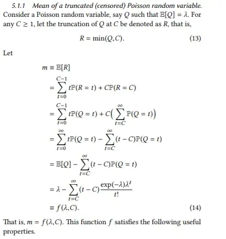
The best way to implement a formula is first to analyze it, because often the way in which it is expressed theoretically is not a good way to compute it. To that end, let's split the sum into two parts:
$$\lambda - f(\lambda,C) = \sum_{t=C}^\infty (t-C) \frac{\exp(-\lambda) \lambda^t}{t!} = e^{-\lambda}\sum_{t=C}^\infty t \frac{\lambda^t}{t!} - e^{-\lambda}\sum_{t=C}^\infty C \frac{\lambda^t}{t!}.$$
For natural numbers $C,$ both of these already look very much like the tail probability for a Poisson$(\lambda)$ variable $X,$
$$S_\lambda(C) = \Pr(X \gt C) =\sum_{t=C+1}^\infty \Pr(X=t)= e^{-\lambda}\sum_{t=C+1}^\infty \frac{\lambda^t}{t!}.$$
Comparing these to the sums in the first formula leads us to re-express them as
$$e^{-\lambda}\sum_{t=C}^\infty t \frac{\lambda^t}{t!} = e^{-\lambda}\sum_{t=C}^\infty \lambda \frac{\lambda^{t-1}}{{t-1}!} = \lambda e^{-\lambda}\sum_{t=C-1}^\infty \frac{\lambda^{t}}{{t}!} = \lambda S_\lambda(C-2)$$
and
$$e^{-\lambda}\sum_{t=C}^\infty C \frac{\lambda^t}{t!} = CS_\lambda(C-1),$$
whence
$$\lambda - f(\lambda,C) = \lambda S_\lambda(C-2) - CS_\lambda(C-1).$$
We should worry a little bit about subtracting one potentially large value from another, which can lose precision, and manipulate this result further to obtain
$$ f(\lambda,C) = \lambda\left(1 - S_\lambda(C-2)\right) + C S_\lambda(C-1) = \lambda F_\lambda(C-2) + C S_\lambda(C-1)$$
where $F_\lambda$ is the Poisson distribution function $F_\lambda(t) = \Pr(X \le t).$ This is a sum of positive values and so will not suffer catastrophic loss of precision.
Any statistical computing platform will provide facilities for quickly and accurately computing $F_\lambda$ and $S_\lambda.$ For instance, an R function to compute $f(\lambda,C)$ is
f <- function(lambda, C) {
  C <- ceiling(C)
  lambda * ppois(C-2,lambda) + C * ppois(C-1, lambda, lower.tail=FALSE)
}
(It uses ppois, which is implemented with an incomplete Gamma function pgamma. See Wikipedia for more.)
Test f through comparison to the brute force summation, such as this quick and dirty implementation based on the definition of $R$.
.f <- Vectorize(function(lambda, C) {
  C <- ceiling(C)
  i <- 0:ceiling(qpois(1 - 1e-15, lambda))
  sum(pmin(i, C) * dpois(i, lambda))
})
Because it sums $O(\lambda)$ terms, it will be inefficient for large $\lambda,$ but that's okay for testing.
A test will compute many values with both functions and study the differences between their outputs, up to reasonably anticipated floating point roundoff error. Here's a quick example that also times the two functions:
lambda <- 2000
C <-  0:ceiling(qpois(1 - 1e-15, lambda))
system.time(a <- f(lambda, C))
system.time(b <-.f(lambda, C))

e <- zapsmall(c(1, b-a))[-1]
plot(a, e)
(The plot shows all the errors are zero.) The benefits of the analysis are clear: where f takes no measurable time, .f takes about one second.
By the way, replacing a variable $Q$ with $R = \min(Q,C)$ is neither "censoring" nor "truncation" in the usual meanings of those terms:
Censoring would replace $Q$ with a category, often written "$\ge C$," whenever $Q \ge C.$ It's usually incorrect to code that category numerically as equal to $C,$ which is what the variable $R$ is doing: that produces biased and often erroneous results when standard procedures are applied.
Truncation would remove all data where $Q \ge C.$ The only possible observations would be the values $0,1,\ldots, C-1.$
Here is an illustration of the distinction. It plots the distribution functions for a truncated, censored, and "censored/truncated" Poisson variable $X$ with $\lambda=7$ and $C=6.$ The left "Truncated" plot attains its maximum value of $1$ by the time $X$ reaches $6$ to reflect the fact that all possible values of $X$ are strictly less than $6.$ The middle "Censored" plot has no values at $6$ and greater because with censoring we simply don't know how the distribution continues.

It is worth knowing these distinctions lest you be led astray by (mistakenly) applying procedures for truncated or censored variables to $R.$

