Is augmentation of treatment effect caused significantly by mediator?

Question

I want to find out if the influence of potential mediator P on treatment effect D is significant. In the two models below $\beta_1$ and $\lambda_1$ are different and I don't know how to test if the difference is significant. Consider D as a perfect random assignment.

$$\hat{y} = \beta_0 + \beta_1D + \epsilon$$

and

$$\hat{y} = \lambda_0 + \lambda_1D + \lambda_2P + \mu$$

I could find a lot of answers comparing differences between two groups. Since I'm considering only one group I think this problem has not been answered before.

I give following example.

Data example

df1 <- structure(list(Y = c(5, 8, 6, 7, 8, 8, 10, 6, 7, 7, 5, 7, 8, 
7, 7, 5, 8, 6, 7, 5, 10, 10, 6, 7, 4, 7, 9, 8, 2, 6, 6, 5, 6, 
6, 6, 7, 6, 4, 7, 2, 6, 5, 8, 7, 5, 6, 6, 8, 6, 6), P = c(5, 
5, 4, 5, 5, 4, 5, 5, 4, 5, 4, 5, 5, 4, 3, 4, 5, 3, 5, 5, 5, 5, 
4, 4, 2, 6, 6, 5, 4, 5, 5, 4, 5, 6, 5, 5, 5, 4, 5, 6, 5, 2, 5, 
4, 4, 5, 5, 6, 4, 5), D = c(0, 0, 0, 0, 0, 0, 0, 0, 0, 0, 0, 
0, 0, 0, 0, 0, 0, 0, 0, 0, 0, 0, 0, 0, 0, 1, 1, 1, 1, 1, 1, 1, 
1, 1, 1, 1, 1, 1, 1, 1, 1, 1, 1, 1, 1, 1, 1, 1, 1, 1)), .Names = c("Y", 
"P", "D"), row.names = c("159.31", "174.31", "106.31", "264.31", 
"424.31", "371.31", "379.31", "399.31", "177.31", "269.31", "133.31", 
"89.31", "78.31", "385.31", "130.31", "330.31", "260.31", "406.31", 
"278.31", "455.31", "245.31", "225.31", "285.31", "173.31", "447.31", 
"310.3", "251.3", "337.3", "122.3", "229.3", "362.3", "241.3", 
"151.3", "140.3", "398.3", "402.3", "169.3", "152.3", "219.3", 
"283.3", "110.3", "359.3", "442.3", "354.3", "415.3", "105.3", 
"246.3", "459.3", "113.3", "161.3"), class = "data.frame")

Models

s0 <- summary(f0 <- lm(Y ~ D , df1))
s1 <- summary(f1 <- lm(Y ~ D + P , df1))
> texreg::screenreg(list(f0, f1))

================================
             Model 1    Model 2 
--------------------------------
(Intercept)   6.96 ***   3.55 **
             (0.32)     (1.14)  
D            -0.96 *    -1.30 **
             (0.46)     (0.43)  
P                        0.77 **
                        (0.25)  
--------------------------------
R^2           0.08       0.24   
Adj. R^2      0.07       0.21   
Num. obs.    50         50      
RMSE          1.61       1.49   
================================
*** p < 0.001, ** p < 0.01, * p < 0.05

Taking P into the model P is significant and D is augmented. Very well. But how can I test if this augmentation is significant?

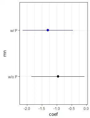
When I plot the coefficients the confidence intervals do overlap.

Plot

m <- rbind(data.frame(var="D", coef=coef(s0)[2, 1], se=coef(s0)[2, 2], mn="w/o P"),
           data.frame(var="D", coef=coef(s1)[2, 1], se=coef(s1)[2, 2], mn="w/ P"))

library(ggplot2)
library(ggstance)
ggplot(m, aes(color=mn)) +
  geom_pointrangeh(aes(y=mn, x=coef, xmin=coef - se*1.96, xmax=coef + se*1.96)) +
  theme_bw() + scale_color_manual(values=c("black", "blue")) +
  guides(color=FALSE)

But I suppose the overlap is not an ultimate proof that there's no significant difference between the two models, though.

An anova() test between both models only would show me if P is significant. But I need to test if the shift of D is significant. How would I do that?

With my real data the AIC difference between both models is $39>2$. According to a "rule of thumb" mentioned in an answer this could be evidence of significant difference. Such a statement would be very thin, though, and I'm not sure.

How can I test if the augmented treatment effect is significant?

Answer 1

The effect of D on Y may be confounded by P. Your second model can be thought of as adjusting for confounding by P. Alternatively, P may be an effect modifier of D on Y. To test for this, test for the interaction of P on D by entering Y~D+P+D*P. In either case, use of the AIC is reasonable to detect the information gain or loss between models. However, you will need to understand the model you built to gain any information from the AIC or other significance tests.