I'm not immediately clear what centroid you want, but the centroid that comes to mind is the point in multivariate space at the centre of the mass of the points per group. About this you want a 95% confidence ellipse. Both aspects can be computed using the ordiellipse() function in vegan. Here is a modified example from ?ordiellipse but using a PCO as a means to embed the dissimilarities in an Euclidean space from which we can derive centroids and confidence ellipses for groups based on the Nature Management variable Management.
require(vegan)
data(dune)
dij <- vegdist(decostand(dune, "log"), method = "altGower")
ord <- capscale(dij ~ 1) ## This does PCO

data(dune.env) ## load the environmental data
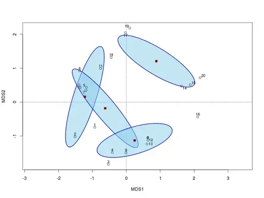
Now we display the first 2 PCO axes and add a 95% confidence ellipse based on the standard errors of the average of the axis scores. We want standard errors so set kind="se" and use the conf argument to give the confidence interval required.
plot(ord, display = "sites", type = "n")
stats <- with(dune.env,
              ordiellipse(ord, Management, kind="se", conf=0.95,
                          lwd=2, draw = "polygon", col="skyblue",
                          border = "blue"))
points(ord)
ordipointlabel(ord, add = TRUE)
Notice that I capture the output from ordiellipse(). This returns a list, one component per group, with details of the centroid and ellipse. You can extract the center component from each of these to get at the centroids
> t(sapply(stats, `[[`, "center"))
         MDS1       MDS2
BF -1.2222687  0.1569338
HF -0.6222935 -0.1839497
NM  0.8848758  1.2061265
SF  0.2448365 -1.1313020
Notice that the centroid is only for the 2d solution. A more general option is to compute the centroids yourself. The centroid is just the individual averages of the variables or in this case the PCO axes. As you are working with the dissimilarities, they need to be embedded in an ordination space so you have axes (variables) that you can compute averages of. Here the axis scores are in columns and the sites in rows. The centroid of a group is the vector of column averages for the group. There are several ways of splitting the data but here I use aggregate() to split the scores on the first 2 PCO axes into groups based on Management and compute their averages
scrs <- scores(ord, display = "sites")
cent <- aggregate(scrs ~ Management, data = dune.env, FUN = mean)
names(cent)[-1] <- colnames(scrs)
This gives:
> cent
  Management       MDS1       MDS2
1         BF -1.2222687  0.1569338
2         HF -0.6222935 -0.1839497
3         NM  0.8848758  1.2061265
4         SF  0.2448365 -1.1313020
which is the same as the values stored in stats as extracted above. The aggregate() approach generalises to any number of axes, e.g.:
> scrs2 <- scores(ord, choices = 1:4, display = "sites")
> cent2 <- aggregate(scrs2 ~ Management, data = dune.env, FUN = mean)
> names(cent2)[-1] <- colnames(scrs2)
> cent2
  Management       MDS1       MDS2       MDS3       MDS4
1         BF -1.2222687  0.1569338 -0.5300011 -0.1063031
2         HF -0.6222935 -0.1839497  0.3252891  1.1354676
3         NM  0.8848758  1.2061265 -0.1986570 -0.4012043
4         SF  0.2448365 -1.1313020  0.1925833 -0.4918671
Obviously, the centroids on the first two PCO axes don't change when we ask for more axes, so you could compute the centroids over all axes once, then use what ever dimension you want.
You can add the centroids to the above plot with
points(cent[, -1], pch = 22, col = "darkred", bg = "darkred", cex = 1.1)
The resulting plot will now look like this
Finally, vegan contains the adonis() and betadisper() functions that are designed to look at differences in means and variances of multivariate data in ways very similar to Marti's papers/software. betadisper() is closely linked to the content of the paper you cite and can also return the centroids for you.