14

I am trying to fit a logistic regression model for business defaults. Apart from the dichotomous variable default, the data set includes some performance ratios. When estimating the model in R, the following warning appears:

glm.fit<-glm(Default~ROS+ROI+debt_ratio,data=ratios,family=binomial)

Warning message:
glm.fit: fitted probabilities numerically 0 or 1 occurred    

However, when I'm using the brglm2 package to detect separation, no separation is detected:

glm.det<-glm(Default~ROS+ROI+debt_ratio,data=ratios,family=binomial("logit"),method="detect_separation")

Separation: FALSE 
Existence of maximum likelihood estimates
(Intercept)         ROS         ROI  debt_ratio 
          0           0           0           0 
0: finite value, Inf: infinity, -Inf: -infinity

And when I'm using the logistf function to penalize complete separation, the variables stop being significant:

glm.adj<-logistf(Default~ROS+ROI+debt_ratio,data=ratios,family=binomial)
logistf(formula = Default ~ ROS + ROI + debt_ratio, data = ratios, 
family = binomial)

Model fitted by Penalized ML
Confidence intervals and p-values by Profile Likelihood Profile Likelihood 
Profile Likelihood Profile Likelihood 

                   coef    se(coef)  lower 0.95   upper 0.95    Chisq          p
(Intercept) -2.10087016 0.134332976 -2.36696659 -1.833575742      Inf 
0.00000000
ROS         -0.01252600 0.009949910 -5.07141750 -0.001546061 5.054069 
0.02456818
ROI         -0.02086535 0.004830609 -0.03171022 -0.012274125 0.000000 
1.00000000
debt_ratio  -0.45693051 0.107951265 -0.69899271 -0.265132585 0.000000 
1.00000000

Likelihood ratio test=53.38183 on 3 df, p=1.519984e-11, n=997
Wald test = 24.06556 on 3 df, p = 2.420494e-05

In case it helps here is the complete set of raw data.

Why doesn't the detect_separation method detect any separation? Is it possible that the variables, even though yielding complete separation, are not at all significant with logistf? How should I proceed?


Update: Added two boxplots (the first one includes all data, while in the second one two outliers are excluded to make the plot slightly clearer), in order to show the dispersion of the data depending on the Default variable.

Boxplot 1 Boxplot 2

Marti
  • 143
  • 1
  • 1
  • 6
  • 2
    I don't know how you're able to see separation in those plots - the points overlap too much to distinguish filled from empty circles in every case. Are you sure the zero/one probabilities aren't just predictions for the observations with extreme predictor values? – Scortchi - Reinstate Monica Mar 24 '18 at 10:04
  • Probably you're right, I'm quite new to this field and have heard about complete separation only recently, thus, maybe I have misinterpreted the plots. I will delete them from the question. But anyway I do not understand whether there is indeed a complete separation, and if yes, why it is not detected? – Marti Mar 24 '18 at 10:27
  • 2
    I don't think you need to delete the marginal model plots - they're useful in suggesting an explanation for the warning message. If there's a value of some predictor below which all responses are 0 & above which all responses are 1 (or vice versa), you do indeed have separation on that predictor. It's simply difficult to see that when points are plotted on top of each other - plot 0's & 1's separately, or just compare the maximum value of the predictor for the 0's with the minimum value for the 1's (or vice versa). – Scortchi - Reinstate Monica Mar 24 '18 at 11:08
  • I added two boxplots, which imho show that, even though there are also some overlapping values, there are some very extreme values of the predictors for Default=1. Does this help? – Marti Mar 24 '18 at 12:23
  • The confidence intervals from logistf do not contain zero. The conflict with what i assume is a Wald test is what I would expect from separation. – mdewey Mar 24 '18 at 12:38
  • I'm not sure if I get what you're saying. The confidence intervals are calculated with the penalized likelihood profile not with the Wald test. Anyway, assuming that there is separation, wouldn't that mean that the predictors are very significant in predicting Default? Why then are their p-values indicating no significance when using the logistf function? – Marti Mar 24 '18 at 14:51
  • Yes, but I assume the chi-squared are Wald tests so what you see is what I would expect from separation. – mdewey Mar 24 '18 at 15:16
  • Ok, I understand that there is indeed a separation problem, but how can I handle it? With glm the coefficients and standard error are elevated on the train set but not if I'm performing glm on the whole set; therefore, it seems to me as if I could not really use the estimates obtained with glm,right? – Marti Mar 24 '18 at 17:10
  • Moreover, I noticed that the coefficients and standard errors are only high when I standardize the variables before; when I do not standardize them, the coefficients and standard errors seem reasonably low to me. Why does standardization blow up the standard errors? – Marti Mar 24 '18 at 17:36
  • 1
    @mdewey: They're supposed to be based on the profile likelihood. Looks like something's gone a bit wappy. Marti: why don't you cross-check using the `brglm` function from `brglm2`, which also penalizes the likelihood according to Firth's method? Your plots don't show separation on any single predictor, & so far there's no reason to distrust the findings from `glm.det`. – Scortchi - Reinstate Monica Mar 24 '18 at 22:18
  • As suggested, I tried the brglmFit function of the brglm2 package. Deviances, AIC and coefficients are not equal but similar. In addition, for some reason the glm function stopped giving me this warning after I used the brglmFit function (however, I am afraid that it will come back, since that happened already once). Would you suggest using only the brglmFit or am I safe to use the glm, which I am more used to? The coefficients (and standard errors in the case of the glm, couldn't find them for the brglmFit) are still high with both function, isn't that kind of a problem? – Marti Mar 24 '18 at 23:00
  • @Scortchi yes, I assumed all that. I do not use logistf so was not 100% sure. – mdewey Mar 25 '18 at 11:06
  • 1
    Why not use predict on the glm output and see which observations are in fact predicted to be zero or unity and then see what covariate values they have? – mdewey Mar 25 '18 at 11:06
  • 1
    As far as what to do next you could do a lot worse than read https://stats.stackexchange.com/questions/11109/how-to-deal-with-perfect-separation-in-logistic-regression especially the answer by @Scortchi – mdewey Mar 25 '18 at 14:02

1 Answers1

18

TL;DR: The warning is not occurring because of complete separation.

library("tidyverse")
library("broom")
# semicolon delimited but period for decimal
ratios <- read_delim("data/W0krtTYM.txt", delim=";")
# filter out the ones with missing values to make it easier to see what's going on
ratios.complete <- filter(ratios, !is.na(ROS), !is.na(ROI), !is.na(debt_ratio))
glm0<-glm(Default~ROS+ROI+debt_ratio,data=ratios.complete,family=binomial)
#> Warning: glm.fit: fitted probabilities numerically 0 or 1 occurred

summary(glm0)
#> 
#> Call:
#> glm(formula = Default ~ ROS + ROI + debt_ratio, family = binomial, 
#>     data = ratios.complete)
#> 
#> Deviance Residuals: 
#>     Min       1Q   Median       3Q      Max  
#> -2.8773  -0.3133  -0.2868  -0.2355   3.6160  
#> 
#> Coefficients:
#>              Estimate Std. Error z value Pr(>|z|)    
#> (Intercept) -3.759154   0.306226 -12.276  < 2e-16 ***
#> ROS         -0.919294   0.245712  -3.741 0.000183 ***
#> ROI         -0.044447   0.008981  -4.949 7.45e-07 ***
#> debt_ratio   0.868707   0.291368   2.981 0.002869 ** 
#> ---
#> Signif. codes:  0 '***' 0.001 '**' 0.01 '*' 0.05 '.' 0.1 ' ' 1
#> 
#> (Dispersion parameter for binomial family taken to be 1)
#> 
#>     Null deviance: 604.89  on 998  degrees of freedom
#> Residual deviance: 372.43  on 995  degrees of freedom
#> AIC: 380.43
#> 
#> Number of Fisher Scoring iterations: 8

When does that warning occur? Looking at the source code for glm.fit() we find

eps <- 10 * .Machine$double.eps
if (family$family == "binomial") {
  if (any(mu > 1 - eps) || any(mu < eps)) 
    warning("glm.fit: fitted probabilities numerically 0 or 1 occurred", 
            call. = FALSE)
}

The warning will arise whenever a predicted probability is effectively indistinguishable from 1. The problem is on the top end:

glm0.resids <- augment(glm0) %>%
  mutate(p = 1 / (1 + exp(-.fitted)),
         warning = p > 1-eps)

arrange(glm0.resids, desc(.fitted)) %>%  
  select(2:5, p, warning) %>% 
  slice(1:10)
#> # A tibble: 10 x 6
#>         ROS      ROI debt_ratio .fitted     p warning
#>       <dbl>    <dbl>      <dbl>   <dbl> <dbl> <lgl>  
#>  1 - 25.0   -10071     452       860    1.00  T      
#>  2 -292     -   17.9     0.0896  266    1.00  T      
#>  3 - 96.0   -  176       0.0219   92.3  1.00  T      
#>  4 - 25.4   -  548       6.43     49.5  1.00  T      
#>  5 -  1.80  -  238      21.2      26.9  1.000 F      
#>  6 -  5.65  -  344      11.3      26.6  1.000 F      
#>  7 -  0.597 -  345       4.43     16.0  1.000 F      
#>  8 -  2.62  -  359       0.444    15.0  1.000 F      
#>  9 -  0.470 -  193       9.87     13.8  1.000 F      
#> 10 -  2.46  -  176       3.64      9.50 1.000 F

So there are four observations that are causing the issue. They all have extreme values of one or more covariates. But there are lots of other observations that are similarly close to 1. There are some observations with high leverage -- what do they look like?

arrange(glm0.resids, desc(.hat)) %>%  
  select(2:4, .hat, p, warning) %>% 
  slice(1:10)
#> # A tibble: 10 x 6
#>        ROS     ROI debt_ratio   .hat     p warning
#>      <dbl>   <dbl>      <dbl>  <dbl> <dbl> <lgl>  
#>  1  0.995  - 2.46      4.96   0.358  0.437 F      
#>  2 -3.01   - 0.633     1.36   0.138  0.555 F      
#>  3 -3.08   -14.6       0.0686 0.136  0.444 F      
#>  4 -2.64   - 0.113     1.90   0.126  0.579 F      
#>  5 -2.95   -13.9       0.773  0.112  0.561 F      
#>  6 -0.0132 -14.9       3.12   0.0936 0.407 F      
#>  7 -2.60   -10.9       0.856  0.0881 0.464 F      
#>  8 -3.41   -26.4       1.12   0.0846 0.821 F      
#>  9 -1.63   - 1.02      2.14   0.0746 0.413 F      
#> 10 -0.146  -17.6       8.02   0.0644 0.984 F

None of those are problematic. Eliminate the four observations that trigger the warning; does the answer change?

ratios2 <- filter(ratios.complete, !glm0.resids$warning)

glm1<-glm(Default~ROS+ROI+debt_ratio,data=ratios2,family=binomial)

summary(glm1)
#> 
#> Call:
#> glm(formula = Default ~ ROS + ROI + debt_ratio, family = binomial, 
#>     data = ratios2)
#> 
#> Deviance Residuals: 
#>     Min       1Q   Median       3Q      Max  
#> -2.8773  -0.3133  -0.2872  -0.2363   3.6160  
#> 
#> Coefficients:
#>             Estimate Std. Error z value Pr(>|z|)    
#> (Intercept) -3.75915    0.30621 -12.277  < 2e-16 ***
#> ROS         -0.91929    0.24571  -3.741 0.000183 ***
#> ROI         -0.04445    0.00898  -4.949 7.45e-07 ***
#> debt_ratio   0.86871    0.29135   2.982 0.002867 ** 
#> ---
#> Signif. codes:  0 '***' 0.001 '**' 0.01 '*' 0.05 '.' 0.1 ' ' 1
#> 
#> (Dispersion parameter for binomial family taken to be 1)
#> 
#>     Null deviance: 585.47  on 994  degrees of freedom
#> Residual deviance: 372.43  on 991  degrees of freedom
#> AIC: 380.43
#> 
#> Number of Fisher Scoring iterations: 6

tidy(glm1)[,2] - tidy(glm0)[,2] 
#> [1]  2.058958e-08  4.158585e-09 -1.119948e-11 -2.013056e-08

None of the coefficients changed by more than 10^-8! So essentially unchanged results. I'll go out on a limb here, but I think that's a "false positive" warning, nothing to worry about. 
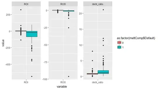
This warning arises with complete separation, but in that case I would expect to see the coefficient for one or more covariates get very large, with a standard error that is even larger. That's not occurring here, and from your plots you can see that the defaults occur across overlapping ranges of all covariates. So the warning occurs because a few observations have very extreme values of the covariates. That could be a problem if those observations were also highly influential. But they're not.

In the comments you asked "Why does standardization blow up the standard errors?". Standardizing your covariates changes the scale. The coefficients and standard errors refer to a one unit change in the covariate, always. So if the variance of your covariate is larger than 1, then standardizing is going to shrink the scale. A one unit change on the standardized scale is the same as a much larger change on the unstandardized scale. So the coefficients and standard errors will get larger. Look at the z values -- they should not change even if you standardize. The z value of the intercept changes if you also center the covariates, because now it is estimating a different point (at the mean of the covariates, instead of at 0)

ratios.complete2 <- mutate(ratios.complete,
                           scROS =  (ROS - mean(ROS))/sd(ROS),
                           scROI =  (ROI - mean(ROI))/sd(ROI),
                           scdebt_ratio = (debt_ratio - mean(debt_ratio))/sd(debt_ratio))
glm2<-glm(Default~scROS+scROI+scdebt_ratio,data=ratios.complete2,family=binomial)
#> Warning: glm.fit: fitted probabilities numerically 0 or 1 occurred
# compare z values
tidy(glm2)[,4] - tidy(glm0)[,4]
#> [1]  4.203563e+00  8.881784e-16  1.776357e-15 -6.217249e-15

Created on 2018-03-25 by the reprex package (v0.2.0).

atiretoo
  • 1,458
  • 14
  • 29
  • 2
    (+1) One quibble: the observations have high *leverage* but aren't "highly influential" - omitting them doesn't change the results much. (In fact you later say they're not influential) – Scortchi - Reinstate Monica Mar 25 '18 at 16:21
  • Yes, good catch. Omitting the four points with highest leverage changes the results much more than the four points triggering the warning, but no qualitative change. – atiretoo Mar 25 '18 at 16:28
  • Any idea what on earth's going on with `logistf`? – Scortchi - Reinstate Monica Mar 25 '18 at 16:32
  • That's a very interesting answer. Which value of eps is correct? I tried `eps – Kevin Zarca Nov 08 '18 at 10:55
  • 1
    I think there is an error in `mutate(p = 1 / (1 + exp(-.fitted))...` - you shouldn't inverse logit the `.fitted`, since it is already a probability after inverse logit transformation. (Assuming that `.fitted` means the same as `glm0$fitted` which is `glm0$fitted.values`, but not sure if I read your dplyr code well since I'm not using it). So it should be `mutate(p = .fitted.values`. Anyway thanks, excellent answer! – Tomas Nov 01 '19 at 22:45
  • So interesting answer! Was having the same warning but am OK – Moses Apr 26 '21 at 12:31