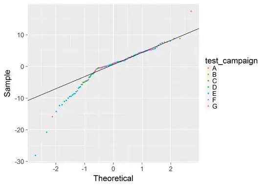
I try to fit several binomial glmms. My interest is wheather historic and recent samples differ in their climatic conditions.
My data is organized as follows, where rand.factI has 62 levels and is nested within rand.factII (9 levels). Binary variable hist_rec is the target variable; it indicates "historic sample" (=0) or "recent sample" (=1). Variables temp.5years and prec.5years are "studentized" (scaled). The table has 379 rows (of which 221 are hist_rec == 1):
> my.data
       rand.factI rand.factII temp.5years  prec.5years   hist_rec
                3           A   2.7762497 -3.178499380          1
               27           B   2.0817516 -2.457070449          0
               27           B   2.0233063 -2.369078844          0
               35           B   2.0315846 -2.229418671          1
               41           A   1.5080735 -1.700811294          1
               93           C   0.4385099  0.162621195          0
               93           C   0.5894258  0.064214693          0
               94           C   0.8763280 -0.044050165          1
               94           C   0.7988891  0.005925186          0
               94           C   0.5989886  0.104371339          0
               94           C   0.3690310  0.230485075          1
              ...         ...         ...          ...        ...
I use the packages
library(lme4)
ibrary(pROC)
My models look like this:
my.model <- glmer(hist_act ~ temp.5years + (1|rand.factI/rand.factII),
            data=my.data, family=binomial)
Outcomes look ok for precipitation, but I have my doubts with the temperature model. Here is a summary of mean values ± standard error for recent and historic sample, p-value of the model, direction of the indicated effect, residual.deviance/residual.degrees.of.freedom (dev_resid) and AUC value.
variable    mean.rec    r.SE mean.hist    h.SE      p  direction  dev_resid signif        AUC
temp.5years     0.77 ± 0.051     -0.55 ± 0.056 0.0000          +       0.29    ***  0.9991122
prec.5years    -0.35 ± 0.089      0.25 ± 0.055 0.0000          -       1.22    ***  0.7806862
dev_resid is << 1 for the temperature model, so I assume that there is some relevant underdispersion. At the same time, the AUC is extremely good - somewhat misleading, I suppose.
The QQ-Plot for the temperature data looks like this:
qqnorm(residuals(my.model, type="deviance"), main=names(compare.data[i]))
qqline(residuals(my.model, type="deviance"), col="green")
abline(a=0, b=1, col="red")
I understand that underdispersion is not possible with binary response variables. In How to handle underdispersion in GLMM (binomial outcome variable), it says:
If you have truly binary, ungroupable outcomes (e.g. one of your response variables is a continuous predictor that is unique to individuals, as would be typical in an observational study), then (1) you can't estimate the degree of overdispersion and (2) you can't really worry about it (i.e., there may be additional sources of variability you don't know about, but they just go to inflate your uncertainty, but they don't bias your inference).
However, the low residual.deviance/residual.degrees.of.freedom - ratio in conjunction with the excellent AUC value make me wonder weather this model is erroneous.
My question is: how should I treat the temperature model? glmer doesn't allow for quasi-families, so I am kind of stuck here. Does it seem promising to transform the temperature variable? Or is there something else I can do to obtain a valid model?
