Replication of results from example in "Econometric Analysis of Panel Data"

Question

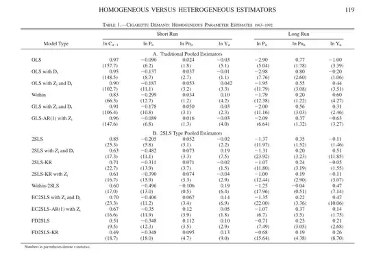
In the textbook Econometric Analysis of Panel Data by Badi H. Baltagi is an example for a dynamic panel data analysis. It is based on the two articles:

Baltagi, Badi H., James M. Griffin, and Weiwen Xiong. "To pool or not to pool: Homogeneous versus heterogeneous estimators applied to cigarette demand." The Review of Economics and Statistics 82.1 (2000): 117-126.

Baltagi, Badi H., and Dan Levin. "Cigarette taxation: raising revenues and reducing consumption." Structural Change and Economic Dynamics 3.2 (1992): 321-335.

I am trying to replicate the results for educational reasons and to get a better understanding of the application of the GMM estimations in R and gretl. The data for the article and the example in the textbook are part of the plm package in R.

One problem I see in the presentation of the results is that there is no intercept in the estimation results, neither in the Baltagi et. al. (2000) article nor in the textbook.

My code to replicate the basic OLS regression:

library(plm)
data("Cigar")
dt.cigar <- data.table(Cigar)

dt.cigar[, `:=`(Real.Price = (price/cpi)
             , Real.GDPpc = (ndi/cpi)
             , Real.Price.Min = pimin/cpi)]

pdata.cigar <- pdata.frame(dt.cigar, index = c("state", "year" ))
# Pooled OLS
summary(plm(log(sales) ~ lag(log(sales), 1) 
    + log(Real.Price)
    + log(Real.Price.Min)
    + log(Real.GDPpc)
#    + factor(year)
    , data= pdata.cigar
    , model="pooling"))
 Pooling Model

Call:
plm(formula = log(sales) ~ lag(log(sales), 1) + log(Real.Price) + 
    log(Real.Price.Min) + log(Real.GDPpc), data = pdata.cigar, 
    model = "pooling")

Balanced Panel: n=46, T=29, N=1334

Residuals :
      Min.    1st Qu.     Median    3rd Qu.       Max. 
-0.2077749 -0.0208569  0.0009819  0.0243556  0.2189800 

Coefficients :
                      Estimate Std. Error  t-value  Pr(>|t|)    
(Intercept)          0.2636862  0.0340032   7.7547 1.752e-14 ***
lag(log(sales), 1)   0.9727864  0.0062527 155.5795 < 2.2e-16 ***
log(Real.Price)     -0.0829222  0.0146180  -5.6726 1.724e-08 ***
log(Real.Price.Min)  0.0160333  0.0130559   1.2280    0.2196    
log(Real.GDPpc)     -0.0322314  0.0062915  -5.1230 3.450e-07 ***
---
Signif. codes:  0 ‘***’ 0.001 ‘**’ 0.01 ‘*’ 0.05 ‘.’ 0.1 ‘ ’ 1

Total Sum of Squares:    67.083
Residual Sum of Squares: 2.3214
R-Squared:      0.96539
Adj. R-Squared: 0.96529
F-statistic: 9268.88 on 4 and 1329 DF, p-value: < 2.22e-16


# Within Estimator
summary(plm(log(sales) ~ lag(log(sales), 1) 
+ log(Real.Price)
+ log(Real.Price.Min)
+ log(Real.GDPpc)

, data= pdata.cigar
, model="within"))
    Oneway (individual) effect Within Model

Call:
plm(formula = log(sales) ~ lag(log(sales), 1) + log(Real.Price) + 
    log(Real.Price.Min) + log(Real.GDPpc), data = pdata.cigar, 
    model = "within")

Balanced Panel: n=46, T=29, N=1334

Residuals :
       Min.     1st Qu.      Median     3rd Qu.        Max. 
-1.7656e-01 -2.1815e-02  5.3382e-05  2.3558e-02  2.3979e-01 

Coefficients :
                      Estimate Std. Error t-value  Pr(>|t|)    
lag(log(sales), 1)   0.8788890  0.0132688 66.2373 < 2.2e-16 ***
log(Real.Price)     -0.1739878  0.0220036 -7.9073 5.632e-15 ***
log(Real.Price.Min)  0.0473236  0.0203675  2.3235   0.02031 *  
log(Real.GDPpc)     -0.0358652  0.0084922 -4.2233 2.577e-05 ***
---
Signif. codes:  0 ‘***’ 0.001 ‘**’ 0.01 ‘*’ 0.05 ‘.’ 0.1 ‘ ’ 1

Total Sum of Squares:    21.514
Residual Sum of Squares: 2.1669
R-Squared:      0.89928
Adj. R-Squared: 0.89543
F-statistic: 2865.95 on 4 and 1284 DF, p-value: < 2.22e-16

The results from the Baltagi et. al. (2000) paper look the following, although the OLS replication is pretty close it's not the same and I don't know what I am missing. I also replicated the results with gretl and I could confirm that the R results are replicable. Does anyone have an idea where the differences might come from? Perhaps differences in the dataset, since there's none of the variables availble, which should be part of the $Z$ vector.

Answer 1

Read the text (text book + variable description in the data set) carefully: "C_it represents real capita sales of cigarettes by persons of smoking age (14 years and older), measured in packs of cigarettes per head". While 14 is an obvious typo (should be 16), it is clear that you are supposed to use the variables pop16 ("population above the age of 16") and pop ("population") from the data set as well.

Also note that the within model in this example is a two-way model ("include time dummies").

Here is what I did to replicate the OLS and within estimates in table 8.1 (numbering as in the 5th ed of the text book):

library(plm)
data("Cigar")
pCigar <- pdata.frame(Cigar)
pCigar$sales16 <- (pCigar$sales*pCigar$pop)/pCigar$pop16

form <- formula(log(sales16) ~ lag(log(sales16), 1) 
                               + log(price/cpi*100)
                               + log(pimin/cpi*100)
                               + log(ndi/cpi*100))

summary(plm(form, data= pCigar, model="pooling"))

## Coefficients :
##                        Estimate Std. Error  t-value  Pr(>|t|)    
## (Intercept)           0.7240693  0.0729962   9.9193 < 2.2e-16 ***
## lag(log(sales16), 1)  0.9694942  0.0061489 157.6687 < 2.2e-16 ***
## log(price/cpi * 100) -0.0901512  0.0145795  -6.1834 8.332e-10 ***
## log(pimin/cpi * 100)  0.0240347  0.0131562   1.8269   0.06794 .  
## log(ndi/cpi * 100)   -0.0306788  0.0060279  -5.0895 4.106e-07 ***
## ....

summary(plm(form, data= pCigar, model="within", effect = "twoways"))

## Coefficients :
##                       Estimate Std. Error  t-value  Pr(>|t|)    
## lag(log(sales16), 1)  0.833383   0.012562  66.3438 < 2.2e-16 ***
## log(price/cpi * 100) -0.298598   0.023601 -12.6519 < 2.2e-16 ***
## log(pimin/cpi * 100)  0.034045   0.027465   1.2396    0.2154    
## log(ndi/cpi * 100)    0.100279   0.023850   4.2046 2.801e-05 ***
## ...

Obviously, some t-statistics in Baltagi's table contain typos (wrong sign), e.g. it is -12.7 (rather than 12.7) for ln(P_it) for the within model.