What is the function computed by this zero inflation model?

Question

Consider this made-up data

require(ggplot2)
require(pscl)
require(visreg)

set.seed(23)
y = c(1005,987,784,1487,0,13,1340,451,0,784,0,451,0,0,123,754, 0, 320,0,12,0,0,87,0,0,0)
d = data.frame(
    y = y,
    x = 1:length(y) + runif(length(y),0,2)
)
ggplot(d, aes(y=y,x=x)) + geom_point() + geom_smooth(method='lm')

I am running a zero inflation model on this data

m = zeroinfl(y~x, dist='negbin', data=d)
print(m)
Call:
zeroinfl(formula = y ~ x, data = d, dist = "negbin")

Count model coefficients (negbin with log link):
(Intercept)            x  
     7.4524      -0.1054  
Theta = 1.181 

Zero-inflation model coefficients (binomial with logit link):
(Intercept)            x  
    -2.3405       0.1453  

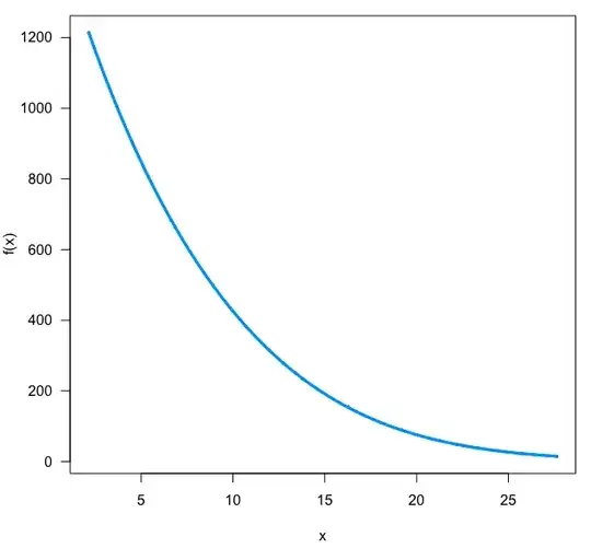
With these four estimates, it should be possible to compute a function to display but I am not sure how. What is my function computed by the zeroinfl function?

When I try to plot the model I get

visreg(m)

Feels about right. What function is this?

Answer 1

The function is simply expectation of the zero-inflation model, see Equation 8 in vignette("countreg", package = "pscl"). This is what ?predict.zeroinfl computes by default (see also Appendix C in the vignette).

To make sure you can try:

visreg(m)
points(d$x, predict(m))

However, the data do not really seem to be count data (or if they are the counts are so large that they are almost continuous). Thus, instead of a zero-inflated count model one could also simply use a Gaussian linear regression, censored at zero (aka tobit model). As pointed out in the post Censored regression in R the model can be fitted with the AER package (interfacing the survreg package) and then one can compute the latent mean, the conditional mean, and the unconditional mean of the response:

library("AER")
fit <- tobit(y ~ x, data = d)
mu <- fitted(fit)
sigma <- fit$scale
p0 <- pnorm(mu/sigma)
lambda <- function(x) dnorm(x)/pnorm(x)
ey0 <- mu + sigma * lambda(mu/sigma)
ey <- p0 * ey0

This yields the following curves for the latent mean (red) and the unconditional mean (blue):

plot(y ~ x, data = d)
abline(fit, col = 2, lwd = 2)
lines(d$x, ey, col = 4, lwd = 2)

A heteroscedastic version of the tobit model is also available in the crch package.