The code you used estimates a logistic regression model using the glm function. You didn't include data, so I'll just make some up.
set.seed(1234)
mydat <- data.frame(
    won=as.factor(sample(c(0, 1), 250, replace=TRUE)),
    bid=runif(250, min=0, max=1000)
)
mod1 <- glm(won~bid, data=mydat, family=binomial(link="logit"))
A logistic regression model models the relationship between a binary response variable and, in this case, one continuous predictor. The result is a logit-transformed probability as a linear relation to the predictor. In your case, the outcome is a binary response corresponding to winning or not winning at gambling and it is being predicted by the value of the wager. The coefficients from mod1 are given in logged odds (which are difficult to interpret), according to:
$$\text{logit}(p)=\log\left(\frac{p}{(1-p)}\right)=\beta_{0}+\beta_{1}x_{1}$$
To convert logged odds to probabilities, we can translate the above to
$$p=\frac{\exp(\beta_{0}+\beta_{1}x_{1})}{(1+\exp(\beta_{0}+\beta_{1}x_{1}))}$$
You can use this information to set up the plot. First, you need a range of the predictor variable:
plotdat <- data.frame(bid=(0:1000))
Then using predict, you can obtain predictions based on your model
preddat <- predict(mod1, newdata=plotdat, se.fit=TRUE)
Note that the fitted values can also be obtained via
mod1$fitted
By specifying se.fit=TRUE, you also get the standard error associated with each fitted value. The resulting data.frame is a matrix with the following components: the fitted predictions (fit), the estimated standard errors (se.fit), and a scalar giving the square root of the dispersion used to compute the standard errors (residual.scale). In the case of a binomial logit, the value will be 1 (which you can see by entering preddat$residual.scale in R). If you want to see an example of what you've calculated so far, you can type head(data.frame(preddat)).
The next step is to set up the plot. I like to set up a blank plotting area with the parameters first:
with(mydat, plot(bid, won, type="n",
    ylim=c(0, 1), ylab="Probability of winning", xlab="Bid"))
Now you can see where it is important to know how to calculate the fitted probabilities. You can draw the line corresponding to the fitted probabilities following the second formula above. Using the preddat data.frame you can convert the fitted values to probabilities and use that to plot a line against the values of your predictor variable.
with(preddat, lines(0:1000, exp(fit)/(1+exp(fit)), col="blue"))
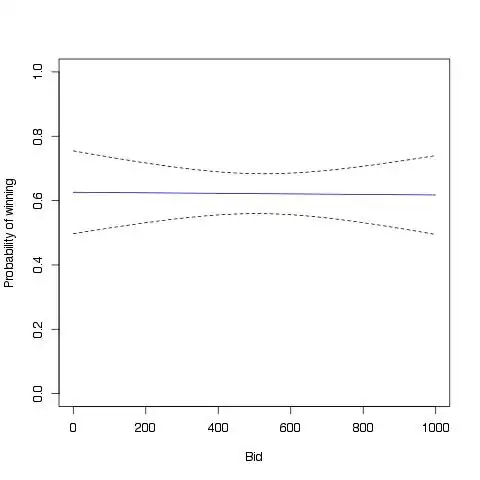
Finally, answer your question, the confidence intervals can be added to the plot by calculating the probability for the fitted values +/- 1.96 times the standard error:
with(preddat, lines(0:1000, exp(fit+1.96*se.fit)/(1+exp(fit+1.96*se.fit)), lty=2))
with(preddat, lines(0:1000, exp(fit-1.96*se.fit)/(1+exp(fit-1.96*se.fit)), lty=2))
The resulting plot (from the randomly generated data) should look something like this:
For expediency's sake, here's all the code in one chunk:
set.seed(1234)
mydat <- data.frame(
    won=as.factor(sample(c(0, 1), 250, replace=TRUE)),
    bid=runif(250, min=0, max=1000)
)
mod1 <- glm(won~bid, data=mydat, family=binomial(link="logit"))
plotdat <- data.frame(bid=(0:1000))
preddat <- predict(mod1, newdata=plotdat, se.fit=TRUE)
with(mydat, plot(bid, won, type="n",
    ylim=c(0, 1), ylab="Probability of winning", xlab="Bid"))
with(preddat, lines(0:1000, exp(fit)/(1+exp(fit)), col="blue"))
with(preddat, lines(0:1000, exp(fit+1.96*se.fit)/(1+exp(fit+1.96*se.fit)), lty=2))
with(preddat, lines(0:1000, exp(fit-1.96*se.fit)/(1+exp(fit-1.96*se.fit)), lty=2))
(Note: This is a heavily edited answer in an attempt to make it more relevant to stats.stackexchange.)