Poisson Regression : expectation vs probability for each outcome

Question

The Poisson regression can be used to predict the expectation count.

e.g: E(number of car | male = 1 & income = 40000) = 1.3

To get this, we can use the predict function in R, e.g:

predict(poisson_model, data, type="response") 

Question:

• How can I get in R the probability of a specific income using the probability mass function? Is there a specific function in Rto do so?

e.g: P(number of car = 0 | male = 1 & income = 40000) = 13%

e.g: P(number of car = 1 | male = 1 & income = 40000) = 28%

Answer 1

If you have a fitted expectation (as you show you can get), using that as a parameter in a Poisson pdf should work.

That is, given $\hat{\lambda}_i = E(Y=0|X=\boldsymbol{x}_i)$ you can use that to calculate whichever probability you want:

$$\hat{P}(Y=k|X=\boldsymbol{x}_i) = \frac{\exp(-\hat{\lambda}_i)\, \hat{\lambda}_i^k}{k!}$$

(In R you'd use dpois() with the parameter set to the fitted mean for that kind of calculation. The process should be about as easy in any number of other packages.)

Answer 2

Just to illustrate the canonical answer by Glen (and with the peace of mind of being late for the party to the point that the answer to the OP has rightfully been adjudicated), let me run a toy example in R, crediting this post also by Glen.

Instead of cars and money, I'll make it more picturesque, and focus on the number of fish caught by a fishing company, in relation to the number of vessels out in the sea - if the numbers seem small, imagine that the units are in $10,000$, or something else. The number of fish caught will follow a Poisson distribution with a rate parameter identical to the number of boats from $\lambda=1$ to $\lambda = 14.$

set.seed(0)
sam = 1000         # Random values from a Pois for each lambda.
lambda = c(1,4,7,10,13) # And these are the lambda values.
x = c(rep(lambda[1], sam), rep(lambda[2], sam), rep(lambda[3], sam), 
      rep(lambda[4], sam), rep(lambda[5],sam)) # These are the number of boats
peixos = rpois(length(x), x)  # And the number of fish caught.

We are establishing a relationship between the expected mean and the $x$ axis strictly linear in this simulation:

$\mathbb E(Y\;\vert\;\text{no. boats})= X\beta + \varepsilon$

but with a Poisson distribution of errors, which parameter changes with the value of the explanatory variable.

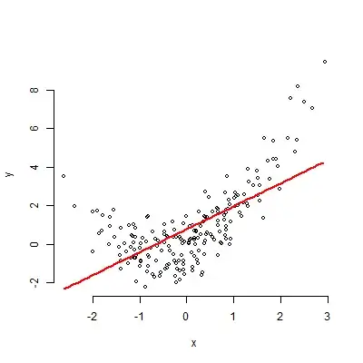
The rate parameter $\lambda$ increases strictly linearly with the number of boats. In the case of a single boat $(\lambda = 1)$ the distribution around the expected mean is manifest in the density of points close to $1$ in the $y$-axis on the plot below - the data points produce a stripped pattern due to the discrete nature of the Poisson distribution. As the value of lambda increases, the distribution of points, and the corresponding histogram, assume more of a normal shape:

The errors (or residuals if you want) are differently spread depending on the number of boats, because we used $5$ different rate parameters. However, once you know the rate parameter for a given value of the explanatory variable, the probability mass function is determined, allowing you to calculate the probability of any other value.

If we tried to recover the lambdas ($\lambda =\{1,4,7,10,13\}$), we'd only have to run the following command:

> fit = glm(peixos ~ x, family = poisson(link = identity))
> unique(predict(fit))
[1]  1.038018  4.023809  7.009600  9.995391 12.981182

Notice that in keeping with the set up of the toy dataset, the rate parameter was linearly dependent with an identity link. The output would have been off if we had run

> fit <- glm(peixos ~ x, "poisson")
> exp(unique(predict(fit)))
[1]  2.270660  3.602671  5.716065  9.069216 14.389387

implicitly using a $\log$ link function - see this post.

---

code here