7

I've downloaded a script to draw a correlation matrix using colored circles. This script allows to order variables using PCA, but I'm not sure how it works. The code responsible for ordering is below:

if (order) {
    if(!n==m){
            stop("The matrix must be squre if order is TRUE!")
    }
  x.eigen <- eigen(corr)$vectors[, 1:2]
  e1 <- x.eigen[, 1]
  e2 <- x.eigen[, 2]
  alpha <- ifelse(e1 > 0, atan(e2/e1), atan(e2/e1) + pi)
  corr <- corr[order(alpha), order(alpha)]
}

Question: What is the interpretation of such ordering and what theory lies behind it?

amoeba
  • 93,463
  • 28
  • 275
  • 317
Tomek Tarczynski
  • 3,854
  • 7
  • 29
  • 37

1 Answers1

9

It is described in Michael Friendly's American Statistician paper on corrgrams, Preprint PDF here. See section on correlation ordering. Also if you look at the source of the corrgram library you will see some other potential ways to order the data as well.

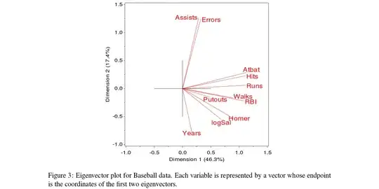
To describe what the code is doing in a nut-shell, the variables in the correlation matrix are ordered according to the correlations with the first and the second principle components extracted from that same correlation matrix. If you look at the Eigenvector plot in the Friendly paper (Figure 3), the code atan(e2/e1) is the angle between the ray associated with a particular variable and the horizontal axis. The variables are sorted by this angle, in a counter-clockwise order. If the whole picture were squeezed horizontally by the square root of the first eigenvalue, and vertically by the square root of the second eigenvalue (this would not change the order!), then the $x$ and $y$ coordinates of each ray's endpoint would be exactly the correlations of this variable with PC1 and with PC2.

Figure 3 from Friendly

Again the reason for the ordering is given in the Friendly paper, but we almost always want more similar things next to more similar things (in either graphics or tables). Frequently the ordering is more informative than the numbers or the graph! Here in this example "more similar" is defined in terms of correlations to the first and the second principle components.

Also note I assume the first if statement in the code prevents this ordering from occurring if the correlation matrix is not full rank.

amoeba
  • 93,463
  • 28
  • 275
  • 317
Andy W
  • 15,245
  • 8
  • 69
  • 191
  • I think your second paragraph does not describe it correctly. E.g. *"the variables in the correlation matrix are ordered according to the correlation with the first principle component"* -- no, not really! For each variable, correlations $c_1$ and $c_2$ with the two first PCs are computed, and then variables are plotted on a 2D plot according to these two coordinates. This is what is used to draw arrows on biplots. Then this procedure orders variables by the angle of the corresponding "biplot arrow". [Also, your second link does not work anymore.] – amoeba Feb 04 '15 at 14:28
  • Maybe I'm confused amoeba, but in the biplot `atan(e2/a1)` is the angle between one ray and the horizontal axis (this of course can be used to figure out the angle to the vertical axis). Isn't the cosine of this angle the correlation between those variables and the first PC? (And subsequently the cosines of the angles between each ray the correlation between those measures?) I will work on the text when I get a chance (replace "ordered based on correlation" to "ordered based on the arccosines of the correlations" or something similar.) – Andy W Feb 04 '15 at 15:22
  • It is unfortunate the second link is not available anymore. Wilkinson and Friendly have a paper, [History of the Cluster Heat Map](http://www.datavis.ca/papers/HeatmapHistory-tas.2009.pdf), which is similar in spirit but I remember the Wilkinson presentation having much more discussion and some analysis of different layouts for heatmaps. – Andy W Feb 04 '15 at 15:25
  • Yes, it's the angle between a ray and the x-axis. The cosine of this angle is not exactly the correlation with the first PC (and the cosines of angles between rays are not exactly the correlations between variables), but are supposed to approximate them. Usually rays represent loadings (i.e. eigenvectors scaled by the square roots of the eigenvalues), and then `e1` and `e2` are exact correlations with the first/second PCs. However, my point was that the ordering is not done based on the correlation with PC1 alone! It's based on the correlations with PC1 and with PC2. – amoeba Feb 04 '15 at 15:32
  • 1
    By the way, your answer could improve a lot if you included a figure (perhaps Figure 3 from Friendly's article); then the explanation becomes much more clear. Note that Friendly does not use loadings for plotting rays, but the eigenvectors themselves. However, it does not seem to matter for ordering, as using loadings would only stretch the whole arrangement horizontally/vertically. – amoeba Feb 04 '15 at 15:33
  • Yes good points amoeba. Not sure when I will get a chance to update with figures (if you rather make your own, more authoritative answer or edit this one feel free.) So in the biplot is the horizontal dimension not the first principal component? (The angle only matters for the ratio of the eigenvectors, so whatever scaling does not matter.) – Andy W Feb 04 '15 at 15:42
  • In a biplot you have variable rays superimposed on a scatter plot of data points. Data points are plotted in PC1 vs PC2 coordinates, i.e. horizontal dimension is PC1 scores, and vertical is PC2 scores. The rays are plotted (usually) such that $(x,y)$ position of each ray endpoint corresponds to $(\rho_1, \rho_2)$ correlations with PC1 and PC2. These correlations are given by loadings, which are eigenvectors scaled by the square roots of eigenvalues. Figure 3 of Friendly shows rays plotted using non-sclaled eigenvectors, so it would need to be squeezed, but differently in hor/vert dimensions. – amoeba Feb 04 '15 at 15:48