If we want to visibly see the distribution of a continuous data, which one among histogram and pdf should be used?
What are the differences, not formula wise, between histogram and pdf?
If we want to visibly see the distribution of a continuous data, which one among histogram and pdf should be used?
What are the differences, not formula wise, between histogram and pdf?
To clarify Dirks point :
Say your data is a sample of a normal distribution. You could construct the following plot:
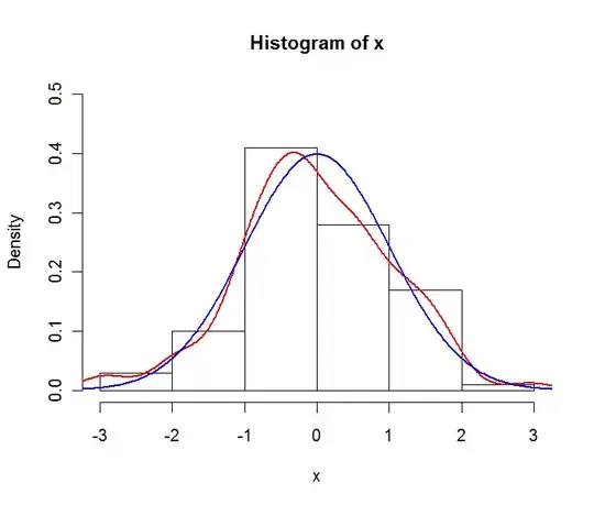
The red line is the empirical density estimate, the blue line is the theoretical pdf of the underlying normal distribution. Note that the histogram is expressed in densities and not in frequencies here. This is done for plotting purposes, in general frequencies are used in histograms.
So to answer your question : you use the empirical distribution (i.e. the histogram) if you want to describe your sample, and the pdf if you want to describe the hypothesized underlying distribution.
Plot is generated by following code in R :
x <- rnorm(100)
y <- seq(-4,4,length.out=200)

hist(x,freq=F,ylim=c(0,0.5))
lines(density(x),col="red",lwd=2)
lines(y,dnorm(y),col="blue",lwd=2)
A histogram is pre-computer age estimate of a density. A density estimate is an alternative.
These days we use both, and there is a rich literature about which defaults one should use.
A pdf, on the other hand, is a closed-form expression for a given distribution. That is different from describing your dataset with an estimated density or histogram.
There's no hard and fast rule here. If you know the density of your population, then a PDF is better. On the other hand, often we deal with samples and a histogram might convey some information that an estimated density covers up. For example, Andrew Gelman makes this point:
A key benefit of a histogram is that, as a plot of raw data, it contains the seeds of its own error assessment. Or, to put it another way, the jaggedness of a slightly undersmoothed histogram performs a useful service by visually indicating sampling variability. That's why, if you look at the histograms in my books and published articles, I just about always use lots of bins. I also almost never like those kernel density estimates that people sometimes use to display one-dimensional distributions. I'd rather see the histogram and know where the data are.
Relative frequency histogram (discrete)
Density Histogram (discrete)
Probability Density Function PDF (continuous)
These references were helpful :) http://stattrek.com/statistics/dictionary.aspx?definition=Probability_density_function
Continuous_probability_distribution from the above site
http://www.geog.ucsb.edu/~joel/g210_w07/lecture_notes/lect04/oh07_04_1.html