Explicitly modelling unequal variances in a linear model to get better conf/pred intervals?

Question

I'm wondering what the best way to generate prediction intervals from a linear model when there is known heteroscedastic AND the heteroscedasticity is predictable.

Consider the following toy example:

   #generate sample data
   sample_df <- data.frame(
        response = c(
            rnorm(50,100,20),
            rnorm(50,20,5)
        ),
        group = c(
            rep("A", 50),
            rep("B", 50)
        )
    )

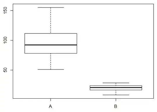
    #Boxplot
    boxplot(response~group, data=sample_df)

An ordinary linear model will give fine spot estimates/predictions for groups A and B, but confidence and prediction intervals will be inappropriate.

Having a look at similar questions on this topic, I've ascertained that gls() from the nlme package can be used to create a model for this situation, but I can't seem to work out how to (easily) generate confidence and prediction intervals from it.

Would this be an appropriate model fit?

gls_1 <- gls(
    response ~ group,
    data = sample_df,
    weights = varIdent(form = ~1|group)
)

Given this model, how would one generate the desired intervals?

score 2 · Accepted Answer · answered Jan 18 '17 at 13:36

See Frank Harrell's package rms:

gls_1 <- gls(
  response ~ group,
  data = sample_df,
  weights = varIdent(form = ~1|group)
)

coef(gls_1)
#Intercept   group=B 
#98.71842 -78.92810 
predict(gls_1, newdata = data.frame(group = c("A", "B")))
#[1] 98.71842 19.79033
#attr(,"label")
#[1] "Predicted values"

library(rms)
gls_2 <- Gls(
  response ~ group,
  data = sample_df,
  weights = varIdent(form = ~1|group),
  B = 1e3 #bootstrap
)
coef(gls_2)
#Intercept   group=B 
#98.71842 -78.92810
Predict(gls_2, group = c("A", "B"))
#group     yhat    lower     upper
#1     A 98.71842 93.50173 103.36231
#2     B 19.79033 18.41493  21.08034
#
#Response variable (y): X * Beta 
#
#Limits are 0.95 confidence limits

Thanks, this gets me halfway there. I'm guessing I'd have to do my own bootstrapping for prediction intervals though? — dcl, Jan 19 '17 at 00:41

score 2 · Answer 2 · answered Jan 18 '17 at 14:16

Roland has a good answer for the CI, but for your first question ("Would this be an appropriate model fit?") I would add that you can check whether this model is more parsimonous than the standard (homogenous variance) model:

# Classic ANOVA (but using the gls function, so models can be compared)
homogenous_var <- gls(
    response ~ group,
    data = sample_df
    )
AIC(homogenous_var, gls_1)

#                df      AIC
# homogenous_var  3 798.0351
# gls_1           4 731.5957

Alternatively, you can use classic hypothesis testing:

anova(homogenous_var, gls_1)

#                Model df      AIC      BIC    logLik   Test  L.Ratio p-value
# homogenous_var     1  3 798.0351 805.7900 -396.0175                        
# gls_1              2  4 731.5957 741.9356 -361.7979 1 vs 2 68.43935  <.0001

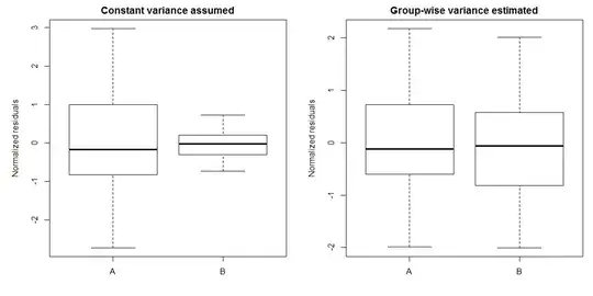
Finally, you can compare standardized residuals for the models:

windows(8,4)
par(mfrow = c(1,2), mar = c(4,5,2,1))

# Standardized residuals from anova
sample_df$homogenous_var_res <- resid(homogenous_var, type = "normalized")
boxplot(homogenous_var_res ~ group, data=sample_df, ylab = "Normalized residuals")

# Standardized residuals from GLS, different variances per group
sample_df$gls_1_res <- resid(gls_1, type = "normalized")
boxplot(gls_1_res~group, data=sample_df, ylab = "Normalized residuals")

Explicitly modelling unequal variances in a linear model to get better conf/pred intervals?

2 Answers2

Linked