How to interpret p=0 in ncvTest?

Question

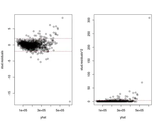
I have constructed a linear model (model3) and I'm trying to check the model's assumptions. As far the assumption of constant variance is concerned I have written the following piece of code

#constant variance
stud.residuals<-rstudent(model3)
yhat<-fitted(model3)
par(mfrow=c(1,2))
plot(yhat,stud.residuals)
abline(h=c(-2,2), col=2,lty=2)
plot(yhat,  stud.residuals^2)
abline(h=4,col=2, lty=2)
ncvTest(model3)
yhat.quantiles<-cut(yhat, breaks=quantile(yhat, prbs=seq(0,1,0.25)), dig.lab=6)
table(yhat.quantiles)
leveneTest(rstudent(model3)~yhat.quantiles)

The output of the above is:

> ncvTest(model3)
Non-constant Variance Score Test 
Variance formula: ~ fitted.values 
Chisquare = 2999.046    Df = 1     p = 0 

> table(yhat.quantiles)
yhat.quantiles
(30917.2,128460]  (128460,167611]  (167611,216345] 
             374              375              375 
 (216345,607215] 
             375 

> leveneTest(rstudent(model3)~yhat.quantiles)
Levene's Test for Homogeneity of Variance (center = median)
        Df F value    Pr(>F)    
group    3  52.424 < 2.2e-16 ***
      1493                      
---
Signif. codes:  0 ‘***’ 0.001 ‘**’ 0.01 ‘*’ 0.05 ‘.’ 0.1 ‘ ’ 1

I'm confused about how to interpret p=0 from ncvTest. At first I thought it would be a matter of representation but ncvTest(model3)$p gives also zero.

Answer 1

pchisq(2999.046, 1, lower.tail = FALSE) gives numerically a 0. You can check pchisq(2999.046, 1, lower.tail = FALSE, log.p = TRUE) to see that the p-value is actually $exp(-150.752) = 3.4e-66$, i.e., a very small probability. However, the exact value is not interesting at all. What this tells you is that there is extremely high significance which means that the zero-hypothesis of constant error variance must be rejected.

Levene's test agrees but formats the printed p-value using format.pval, i.e., shows it as smaller than a value roughly corresponding to precision of floating point numbers.

Finally, formal tests are nice, but it's usually recommended to focus on the diagnostic plots. And those show you heterogeneity and hint at systematic underestimation for lower fitted values and overestimation for the middle range.