Generate two variables with heteroscedastic residuals and a linear regression slope of 1

Question

I have a vector A, which comprises predefined revenue values of 1000 companies. Now I want to generate another vector B, which comprises the companies' revenue of the previous year. The intention is to model B by taking A as the expected value and a standard deviation that increases with the size of A: That is, larger companies have larger absolute differences between A and B than smaller companies. The purpose is to achieve a relation so that a linear regression of the predictor B on the dependent variable A would yield a line with a slope of close to 1. Hence, the relation should look as follows:

lm(A~B)$coefficients  # should yield  
                      #(Intercept)          B 
                      #     0               1
plot(B,A)
abline(lm(A~B)$coefficients, col = "red")`

I tried it as follows:

set.seed(123)
A <- 1:1000
B <- rnorm(n=1000, mean = A, sd=0.4*A)

However, for lm(A~B):

Coefficients:
(Intercept)          A
197.5979             0.6013

Do you have any idea how I can fix the generation of vector B from A, so that a linear regression of B on A would yield a slope of 1?

Does it have to be *exactly* one or is approximately (like 1.0076) good enough? — Christoph Hanck, Nov 14 '16 at 12:26
Approximately like 1.0076 is definitely enough. However, it is important that B is the predictor and A the dependent variable and that B has to be generated from A before. — Julia236, Nov 14 '16 at 12:33
Do you want to include the possibility of negative revenues in your simulation? Note that you have them now. Although I don't work in economics or business, I wouldn't think of revenues as being normally distributed, but probably something skewed & w/ fat tails. — gung - Reinstate Monica, Nov 14 '16 at 17:27

Bad John · Answer 1 · 2016-11-14T13:02:49.460

3

In order to take an estimate for $b$ equal to one you have to change the standard deviation. I used your code and I just changed it. Look at this:

set.seed(123)
A <- 1:1000
B <- rnorm(n=1000, mean = A, sd=1/A)

lm(A~B)

    Call:
lm(formula = A ~ B)

Coefficients:
(Intercept)            B  
 -0.0003096    1.0000004

lm(B~A)

Call:
lm(formula = B ~ A)

Coefficients:
(Intercept)            A  
  0.0003144    0.9999996

I suppose that this is what you want. Note that you will take similar results in case of using standard deviation $sd = A^k$, for each $k$ not zero of course.

edited Nov 14 '16 at 13:02

answered Nov 14 '16 at 12:56

Bad John

145
6

Thank you a lot for your reply and adjustment! However, the purpose is that the standard deviation of B increases with A as displayed in the illustration above. With your hint of sd=1/A, the opposite is the case. My fault, I probably didn't make that intention clear enough and will edit it in the question. I also tried sd=A^k, with (among others) k=0.8, which lead to the same problem of lm(A~B) yielding a slope of far below 1. – Julia236 Nov 14 '16 at 16:00

score 0 · Accepted Answer · edited Apr 13 '17 at 12:44

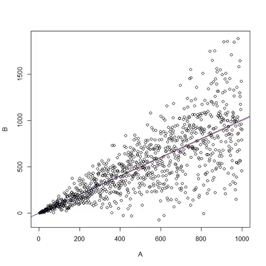
You're almost there. The thing you need to remember is that regression minimizes the vertical distances of the data to the line. That is, we think of the errors as being in the response (see my answer here: What is the difference between linear regression on y with x and x with y?). You just need to switch around which variable is your response here. Consider:

set.seed(123)
A <- 1:1000
B <- rnorm(n=1000, mean = A, sd=0.4*A)
summary(lm(A~B))$coefficients  # this is your regression
#                Estimate Std. Error  t value      Pr(>|t|)
# (Intercept) 197.5978552 9.62892402 20.52128  2.361529e-78
# B             0.6012796 0.01535132 39.16794 5.465950e-204
summary(lm(B~A))$coefficients
#               Estimate  Std. Error     t value      Pr(>|t|)
# (Intercept) -0.5542773 14.86392934 -0.03729009  9.702612e-01
# A            1.0076260  0.02572579 39.16793538 5.465950e-204

windows()
  # plot(B,A)  # this is your plot
  plot(A,B)    # here I switched X & Y
  abline(0,1, col="red")
  abline(coef(lm(B~A)), col="blue")

Generate two variables with heteroscedastic residuals and a linear regression slope of 1

2 Answers2