I have a data frame called mxDF looks like this:
> head(mxDF)
     y x.Age x.Weight x.Height x.Medicine x.genotype1
1 3.00    36       72      171                  0                    0
2 1.50    63       49      162                  0                    0
3 2.25    40       44      154                  0                    0
4 2.25    57       41      159                  0                    0
5 2.25    59       55      157                  0                    0
6 1.50    45       51      160                  0                    0
  x.genotype2
1                      0
2                      0
Then I did the following:
mxMod     <- glm(mxDF)
res.mxMod <- resid(mxMod);
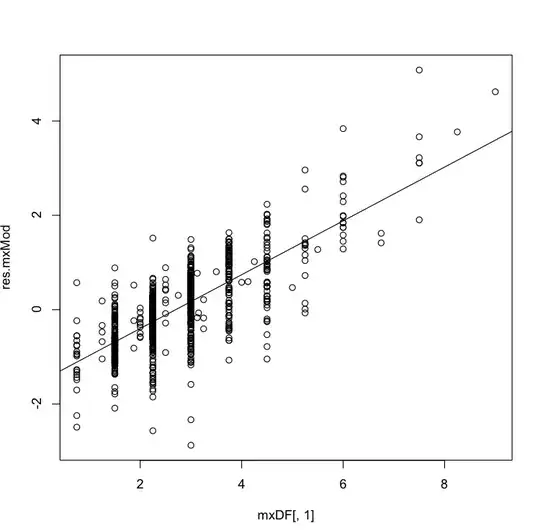
plot(res.mxMod ~ mxDF[,1]);
abline(glm(res.mxMod ~ mxDF[,1]))
And the plot looks like below:
The pattern on the residue plot is so obvious, and then I did a glm on the residue ~ outcome:
summary(glm(res.mxMod ~ mxDF[,1]))
Call:
glm(formula = res.mxMod ~ mxDF[, 1])

Deviance Residuals:
     Min        1Q    Median        3Q       Max
-3.04479  -0.28613   0.03926   0.36334   2.34211

Coefficients:
            Estimate Std. Error t value Pr(>|t|)
(Intercept) -1.54024    0.04782  -32.21   <2e-16 ***
mxDF[, 1]    0.57049    0.01630   34.99   <2e-16 ***
---
Signif. codes:  0 ‘***’ 0.001 ‘**’ 0.01 ‘*’ 0.05 ‘.’ 0.1 ‘ ’ 1

(Dispersion parameter for gaussian family taken to be 0.3229295)

    Null deviance: 693.21  on 923  degrees of freedom
Residual deviance: 297.74  on 922  degrees of freedom
AIC: 1581.8

Number of Fisher Scoring iterations: 2
Isn't this weird? What did I do wrong?
