4

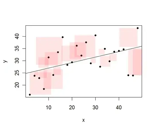
I came across this nice illustration of the "Coefficient of determination" (source):

enter image description here

Which leads me to ask two questions:

  1. How to do it with R? (I guess my main question would be how to deal with the opacity)
  2. Are there other interesting/useful visualizations of the "Coefficient of determination"? (and again, is there an easy way to make them in R?)

Thanks.

chl
  • 50,972
  • 18
  • 205
  • 364
Tal Galili
  • 19,935
  • 32
  • 133
  • 195
  • Just curious, where did you find that illustration? –  Feb 25 '12 at 16:30
  • I forgot to link, here is the source: http://en.wikipedia.org/wiki/File:Coefficient_of_Determination.svg – Tal Galili Feb 25 '12 at 16:52
  • 2
    re #2: A different graphical method to explain covariance (and therefore, in an obvious way, the correlation coefficient) appears at http://stats.stackexchange.com/a/18200. However, I used *Mathematica* to make the illustration, not R, and even *Mathematica* could not quite do what I wanted (which is to get complementary overlapping colors to cancel rather than add). – whuber Feb 25 '12 at 18:10

1 Answers1

7

In R, use the alpha argument to hsv():

# Create test data.
# (These parameters produce a bunch of multiple overlaps.)
set.seed(17)
x <- (1:24)*2
y <- 24 + x/8 + 8 * rnorm(length(x))

# Draw the figure.
plot(x, y, pch=19, cex=0.8)   # Plot the points
fit <- lm(y ~ x)              # Find the least squares line
abline(fit)                   # Plot the line
u <- mapply(function(x,y,r) rect(x, y, x-r, y-r, col=hsv(1,alpha=0.1), border=NA), 
     x, y, fit$residuals)     # Plot the squares

Covariance plot

whuber
  • 281,159
  • 54
  • 637
  • 1,101