Options for quantifying changes in the functional form of a response curve

Question

I've inherited observations of a response variable ($y$) measured over time ($t$) during which the response increases and subsequently decreases. The measurement of this response occurs repeatedly over ~ 50 replications ($rep$). The code below pulls in some data from six example $rep$s spanning the range of the replicates. In this case, time $t$ has been centered across all $rep$s but it need not be.

Some complications of the data include, as the figure illustrates, that the response is usually not measured until after is underway and before the decline has concluded. This is especially true in later replicates, which observe a smaller window and make fewer measurements of the response curve (e.g., see $rep$ 6).

tmp <- tempfile()
download.file("https://gist.githubusercontent.com/adamdsmith/cbb8fa530fa6f1f9c32e41be487ded63/raw/18d3ccf205df181a6343712798b384ecf71dbc27/data.R", tmp)
source(tmp)
library("ggplot2")
ggplot(dat, aes(t,y,group = rep, colour = rep)) + geom_line(size=1) + 
  geom_point() + theme_classic()

The problem

I want to quantify changes in the response function over replicates, most notably whether:

1. the temporal location of the maximum response (i.e., the $t$ of peak $y$) changes consistently over $rep$s, and

2. the shape of the response curve, particularly its width at some standardized level of response $y$, also changes as a function of $rep$ (i.e., is the response curve becoming more protracted or abbreviated over $rep$s?). This may be too simplistic, and other parameters describing the response curve may be worth considering (e.g., skew, kurtosis, etc.).

What makes the most intuitive sense is to assume a single underlying response function that describes the mean change in $y$ over $t$ and then evaluate whether the parameters describing this function vary over $rep$. This "hierarchical" structure can then be evaluated readily in a Bayesian framework. The actual height of the curve in each $rep$ is, for various reasons, not of interest and thus variability in any related parameter(s) is preferentially be captured with a random $rep$ effect.

Options considered thus far

There's no shortage of possible ways to model this response function and its change with $rep$, but each approach that I've considered has apparent shortcomings and I'm mentally stuck on a reasonable way forward:

1. Quadratic function

   This seems an easy way to get at the questions, particularly using the vertex form: $y = a(t - h)^2 + c$, where $a$ controls the width of the parabola (and the direction it opens), $h$ controls the horizontal position of the vertex, and both can be modeled as a function of $rep$. $c$ controls the vertical position of the vertex and is easily captured with a random effect. Unfortunately, this approach assumes symmetry about the peak response, which doesn't hold as the decline after peak response seems to occur more quickly than the increase (see, e.g., $rep$s 2-4).

2. Gaussian function

   Another relatively easy way, where $y = ae^{-\frac{(t - m)^2}{2s^2}}$ and $a$ controls the height of curve's peak, $m$ controls the horizontal ($t$) position of peak (mean), and $s$ controls width of curve (standard deviation). But this form has the same symmetry problem as the quadratic function. Certainly Guassian functions can incorporate various degrees of skew and kurtosis but I don't think there's an easy way to model these aspects without cumulative distribution functions/integration.

3. Trigonometric regression (sine/cosine Fourier terms)

   Trigonometric functions based on $sin$/$cos$ pairs are another relatively easy option (see, e.g., here). The first $sin$/$cos$ pair terms produces a symmetric sine wave, but additional $sin$/$cos$ pairs with different functional periods get past this limitation. Unfortunately, what experimentation I've done suggests it takes several additional $sin$/$cos$ pairs of unknown period (i.e., need to be estimated) to adequately capture the asymmetry, which quickly gets unwieldy and yields inadequate fits in some $rep$s.

4. Additive models/smoothing splines

   An additive model seems to get around many of these limitations, but then I lose the seemingly preferable state of having a fixed underlying response function defined by parameters than I can allow to vary with increasing $rep$. Would a factor-smooth interaction that forced the smooth for each $rep$ to have the same smoothing parameter be a reasonable compromise? For example, something like:

   library(mgcv)
   ?factor.smooth.interaction
   m <- gam(y ~ s(t, rep, bs = "fs"), data = dat)
   plot(m)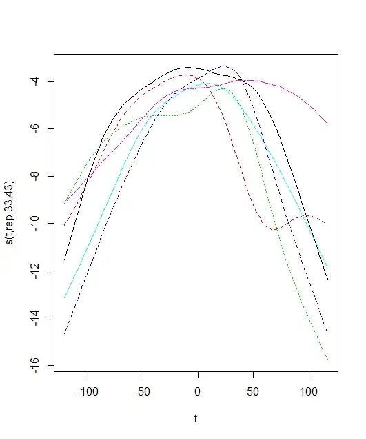
   

   

   If this is a reasonable solution, how then can I relate the peak or the width of each smooth to $rep$? Finding the peak of fitted smooths is a relatively simple exercise (see here), but is it reasonable to then model these derived values (and uncertainty) as a function of $rep$ in a separate model?

Thanks very much for considering. As is likely obvious, I'm most comfortable with R, but I'm open to any solutions.