34

I want to generate the plot described in the book ElemStatLearn "The Elements of Statistical Learning: Data Mining, Inference, and Prediction. Second Edition" by Trevor Hastie & Robert Tibshirani& Jerome Friedman. The plot is:

enter image description here

I am wondering how I can produce this exact graph in R, particularly note the grid graphics and calculation to show the boundary.

chl
  • 50,972
  • 18
  • 205
  • 364
littleEinstein
  • 523
  • 1
  • 5
  • 7
  • 4
    Is it this one: http://www-stat.stanford.edu/~tibs/ElemStatLearn/datasets/mixture.example.info ? – StasK Jan 24 '12 at 01:42

2 Answers2

36

To reproduce this figure, you need to have the ElemStatLearn package installed on you system. The artificial dataset was generated with mixture.example() as pointed out by @StasK.

library(ElemStatLearn)
require(class)
x <- mixture.example$x
g <- mixture.example$y
xnew <- mixture.example$xnew
mod15 <- knn(x, xnew, g, k=15, prob=TRUE)
prob <- attr(mod15, "prob")
prob <- ifelse(mod15=="1", prob, 1-prob)
px1 <- mixture.example$px1
px2 <- mixture.example$px2
prob15 <- matrix(prob, length(px1), length(px2))
par(mar=rep(2,4))
contour(px1, px2, prob15, levels=0.5, labels="", xlab="", ylab="", main=
        "15-nearest neighbour", axes=FALSE)
points(x, col=ifelse(g==1, "coral", "cornflowerblue"))
gd <- expand.grid(x=px1, y=px2)
points(gd, pch=".", cex=1.2, col=ifelse(prob15>0.5, "coral", "cornflowerblue"))
box()

All but the last three commands come from the on-line help for mixture.example. Note that we used the fact that expand.grid will arrange its output by varying x first, which further allows to index (by column) colors in the prob15 matrix (of dimension 69x99), which holds the proportion of the votes for the winning class for each lattice coordinates (px1,px2).

enter image description here

chl
  • 50,972
  • 18
  • 205
  • 364
  • +1. thanks! I am also wondering how to generate the data as described in the text "expose the oracle". Could you also please add that, instead of using the data from the website? – littleEinstein Jan 24 '12 at 19:32
  • @littleEinstein Do you mean what is given in the on-line help for `mixture.example`? Look at the simulation setup below line starting with `# Reproducing figure 2.4, page 17 of the book:` in the example section. – chl Jan 24 '12 at 20:12
  • can you please let me know the link? I cannot find it. – littleEinstein Jan 24 '12 at 20:51
  • Sorry @littleEinstein, but there's something I'm probably missing. It is just a matter of typing `help(mixture.example)` or `example(mixture.example)` at R prompt (after you load the required package with `library(ElemStatLearn)`). The code to generate the artificial dataset (not to generate Fig. 2.4) is written in plain R in the Example section. – chl Jan 24 '12 at 21:03
  • If I am not mistaken, the code there in the Example section actually references the data set, rather than generating it from scratch. I am talking about how to generate the dataset `mixture.example` itself. Really thank you for your help! – littleEinstein Jan 24 '12 at 23:31
  • That's right. This is only a data structure (a similar one can be found in the [mda](http://cran.r-project.org/web/packages/mda/index.html) package). I would have thought the description in the book on how to generate the dataset would have been clear enough for implementing it. You can ask for confirmation, but really the code in the on-line doc should help approximating data found in `mixture.example` (the only fact that is missing is that we don't what seed they used). – chl Jan 25 '12 at 12:20
  • 1
    BTW, I just came across @Shane's weblog where he used `ggplot` for similar purpose. Check this out: [ESL 2.1: Linear Regression vs. KNN](http://www.statalgo.com/2011/04/24/esl-2-1-linear-regression-vs-knn/). – chl Feb 25 '12 at 18:56
7

I'm self-learning ESL and trying to work through all examples provided in the book. I just did this and you can check the R code below:

library(MASS)
# set the seed to reproduce data generation in the future
seed <- 123456
set.seed(seed)

# generate two classes means
Sigma <- matrix(c(1,0,0,1),nrow = 2, ncol = 2)
means_1 <- mvrnorm(n = 10, mu = c(1,0), Sigma)
means_2 <- mvrnorm(n = 10, mu = c(0,1), Sigma)

# pick an m_k at random with probability 1/10
# function to generate observations
genObs <- function(classMean, classSigma, size, ...)
{
  # check input
  if(!is.matrix(classMean)) stop("classMean should be a matrix")
  nc <- ncol(classMean)
  nr <- nrow(classMean)
  if(nc != 2) stop("classMean should be a matrix with 2 columns")
  if(ncol(classSigma) != 2) stop("the dimension of classSigma is wrong")

  # mean for each obs
    # pick an m_k at random
  meanObs <- classMean[sample(1:nr, size = size, replace = TRUE),]
  obs <- t(apply(meanObs, 1, function(x) mvrnorm(n = 1, mu = x, Sigma = classSigma )) )
  colnames(obs) <- c('x1','x2')
  return(obs)
}


obs100_1 <- genObs(classMean = means_1, classSigma = Sigma/5, size = 100)
obs100_2 <- genObs(classMean = means_2, classSigma = Sigma/5, size = 100)

# generate label
y <- rep(c(0,1), each = 100)

# training data matrix
trainMat <- as.data.frame(cbind(y, rbind(obs100_1, obs100_2)))

# plot them
library(lattice)
with(trainMat, xyplot(x2 ~ x1,groups = y, col=c('blue', 'orange')))

# now fit two models

# model 1: linear regression
lmfits <- lm(y ~ x1 + x2 , data = trainMat)

# get the slope and intercept for the decision boundary
intercept <- -(lmfits$coef[1] - 0.5) / lmfits$coef[3]
slope <- - lmfits$coef[2] / lmfits$coef[3]

# Figure 2.1
xyplot(x2 ~ x1, groups = y, col = c('blue', 'orange'), data = trainMat,
       panel = function(...)
       {
        panel.xyplot(...)
        panel.abline(intercept, slope)
        },
       main = 'Linear Regression of 0/1 Response')    

# model2: k nearest-neighbor methods
library(class)
# get the range of x1 and x2
rx1 <- range(trainMat$x1)
rx2 <- range(trainMat$x2)
# get lattice points in predictor space
px1 <- seq(from = rx1[1], to = rx1[2], by = 0.1 )
px2 <- seq(from = rx2[1], to = rx2[2], by = 0.1 )
xnew <- expand.grid(x1 = px1, x2 = px2)

# get the contour map
knn15 <- knn(train = trainMat[,2:3], test = xnew, cl = trainMat[,1], k = 15, prob = TRUE)
prob <- attr(knn15, "prob")
prob <- ifelse(knn15=="1", prob, 1-prob)
prob15 <- matrix(prob, nrow = length(px1), ncol = length(px2))
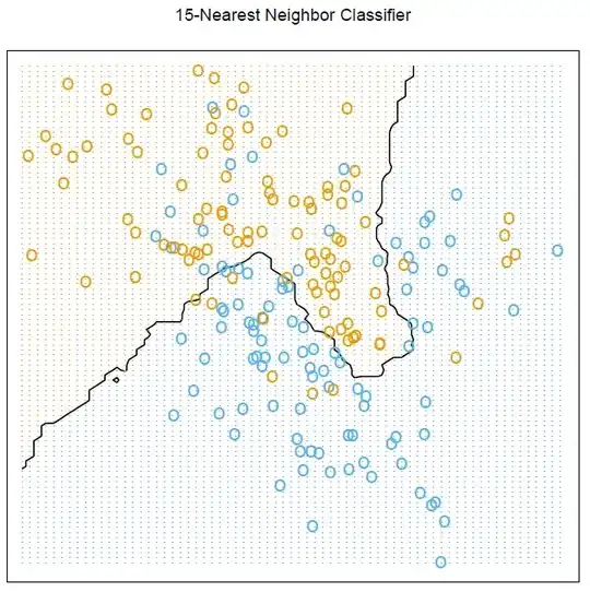
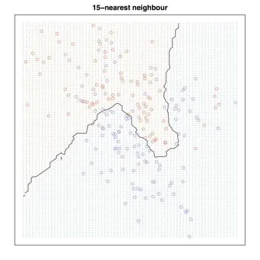
# Figure 2.2
par(mar = rep(2,4))
contour(px1, px2, prob15, levels=0.5, labels="", xlab="", ylab="", main=
    "15-nearest neighbour", axes=FALSE)
points(trainMat[,2:3], col=ifelse(trainMat[,1]==1, "coral", "cornflowerblue"))
points(xnew, pch=".", cex=1.2, col=ifelse(prob15>0.5, "coral", "cornflowerblue"))
box()
Daoying Lin
  • 71
  • 1
  • 1