Max Entropy Solver in R

Question

I am trying to solve for the parameters in the maximum entropy problem in R using the nonlinear system:

$\ \int_l^u e^{a+bx+cx^2}dx=1$

$\ \int_l^u x e^{a+bx+cx^2}dx=\mu$

$\ \int_l^u x^2 e^{a+bx+cx^2}dx=\mu^2+\sigma^2$

where $l$ and $u$ represent the lower and upper bound on the support of the distribution, and $a,b,c$ are the parameters of interest.

I wrote an implementation based on minimising the sum of the squared differences, and then optimising using BBoptim, but this method is very hit-or-miss, and depends heavily upon me inputting reasonable starting parameters, and quite tight lower and upper bounds on the range over which to search. I have included the code below:

MaxEnt <- function(y) {
G <- function(x) exp(y[1]+y[2]*x+y[3]*x^2) ;
H <- function(x) x*exp(y[1]+y[2]*x+y[3]*x^2) ;
I <- function(x) x^2*exp(y[1]+y[2]*x+y[3]*x^2) ;
(integrate(G, lower=l, upper=u)$value - 1)^2+(integrate(H, lower=l, upper=u)$value - mu)^2+(integrate(I, lower=l, upper=u)$value - mu^2-sd^2)^2}
BBoptim(c(-log(sqrt(2*pi)),0,0), MaxEnt, method=1)

Does anyone know of any better ways of doing what I am trying to achieve using R? Many thanks in advance.

============ EDIT JAN 17th ============

I have tried solving this problem using whuber's approach and so far this is what I get:

Let $\ y= \frac{x-l}{u-l}$. Then $\ dx = (u-l)dy$. Then since $\ x= (u-l)y+l$,

$\ a+bx+cx^2 = q+ry+cy^2$

where $\ q=a+bl+cl^2,r=(u-l)(b+2cl),s=c(u-l)^2$. The three original equations then become:

$\ \int_0^1 e^{q+ry+sy^2}dy=\frac{1}{u-l}$

$\ \int_0^1 ((u-l)y+l) e^{q+ry+sy^2}dy=\frac{\mu}{u-l}$

$\ \int_0^1 ((u-l)y+l)^2 e^{q+ry+sy^2}dy=\frac{\mu^2+\sigma^2}{u-l}$

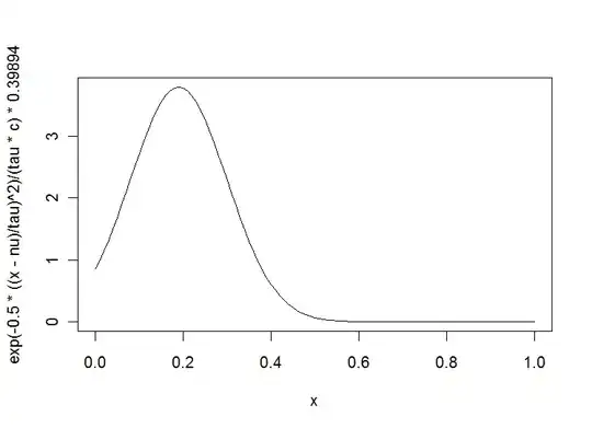
whuber then suggests rewriting $\ e^{q+ry+sy^2}$. Letting $\ \nu = \frac{-r}{2s}$ and $\ \tau = \sqrt{\frac{-1}{2s}}$ we can see that $\ e^{q+ry+sy^2} = e^{q-\frac{r^2}{2s}}e^{-0.5\left(\frac{y-\nu}{\tau}\right)^2}$.

The problem I now have is that using whubers approach we must have that $\ \tau^2 >0 $ (?). This means I need $\ s<0$. By definition, $\ s <0$ only if $\ c <0$ also. However, I have an example where the density that has maximum entropy has $c>0$. I am probably going wrong somewhere, and would be grateful if somebody could point out where. Thanks!

Answer 1

Making the change of variables $x = l + (u-l)y$ puts the problem into the same form with $u=1, l=0$. Rewrite the density in the form $f(x,\nu,\tau)=\exp(-1/2((x-\nu)\tau)^2)/(\sqrt{2\pi}\tau)$ and rewrite the equations as

$$\eqalign{ \int_0^1 x f(x,\nu,\tau) dx &= \mu \int_0^1 f(x,\nu,\tau)\\ \int_0^1 x^2 f(x,\nu,\tau)dx &= (\mu^2+\sigma^2) \int_0^1 f(x,\nu,\tau). }$$

All three integrals can be written explicitly in terms of the exponential exp and the cumulative standard normal distribution pnorm. This suggests the following R code for the core calculations; straightforward algebraic manipulations will produce the desired values of $a$, $b$, and $c$:

f0 <- function(x){ # Normalization factor
    mu<-x[1];sigma<-x[2]
    pnorm((1-mu)/sigma)-pnorm(-mu/sigma)
}
f1 <- function(x){ # First moment
    mu<-x[1];sigma<-x[2]
    (-exp(-0.5*((1-mu)/sigma)^2)+exp(-0.5*(mu/sigma)^2))*sigma*0.39894228040143268 + mu * f0(x)
}
f2 <- function(x){ # Second moment
    mu<-x[1];sigma<-x[2]
    (-(1+mu)*exp(-0.5*((1-mu)/sigma)^2)+mu*exp(-0.5*(mu/sigma)^2))*sigma*0.39894228040143268 + (mu^2+sigma^2) * f0(x)
}
f <- function(x,y){ # Discrepancy between first two moments determined by parameters x and target values (y)
    mu<-y[1];sigma<-y[2]
    c<-f0(x)
    (mu-f1(x)/c)^2 + (mu^2+sigma^2-f2(x)/c)^2
}
fit <- function(mu, sigma) {
    # Computes a truncated normal distribution on [0,1] with mean mu and SD sigma
    #     (the "max ent" solution--but see the comments). 
    # NB: naively takes (mu,sigma) as starting values.
    optim(c(mu,sigma), function(x){f(x,c(mu,sigma))})
}

As an example of running and checking this code, consider the problem with $\mu=0.2$, $\sigma=0.1$:

> mu <- .2
> sigma <- .1
> z <- fit(mu, sigma)
> z$par
[1] 0.1897255 0.1097969
> f1(z$par) / f0(z$par) # Should equal mu
0.2000000
> mu^2 + sigma^2
.05
> f2(z$par) / f0(z$par) # Should equal mu^2 + sigma^2
0.05000045
> nu <- z$par[1]
> tau <- z$par[2]
> gamma <- f0(z$par)
> curve(exp(-0.5*((x-nu)/tau)^2)/(tau*gamma) * 0.39894, 0, 1)

As required, this is a truncated normal distribution with the desired mean and variance. Shift and rescale it to arbitrary intervals $[l,u]$ as needed. This example was easy--the truncated distribution is close to normal anyway--but you will find that more extreme examples (such as $(\mu,\sigma)=(0.1,0.4)$) work just fine. (The speed is reasonable, too: on my system fit is taking 4 to 7 milliseconds.)