9

Let's say that I generate the probability of an outcome based on a certain factor and plot the curve of that outcome. Is there any way to extract the equation for that curve from R?

> mod = glm(winner~our_bid, data=mydat, family=binomial(link="logit"))
> summary(mod)

Call:
glm(formula = winner ~ our_bid, family = binomial(link = "logit"), 
    data = mydat)

Deviance Residuals: 
    Min       1Q   Median       3Q      Max  
-0.7443  -0.6083  -0.5329  -0.4702   2.3518  

Coefficients:
              Estimate Std. Error z value Pr(>|z|)    
(Intercept) -9.781e-01  2.836e-02  -34.49   <2e-16 ***
our_bid     -2.050e-03  7.576e-05  -27.07   <2e-16 ***
---
Signif. codes:  0 ‘***’ 0.001 ‘**’ 0.01 ‘*’ 0.05 ‘.’ 0.1 ‘ ’ 1 

(Dispersion parameter for binomial family taken to be 1)

    Null deviance: 42850  on 49971  degrees of freedom
Residual deviance: 42094  on 49970  degrees of freedom
AIC: 42098

Number of Fisher Scoring iterations: 4

> all.x <- expand.grid(winner=unique(winner), our_bid=unique(our_bid))
> all.x
> won = subset(all.x, winner == 1)
> y.hat.new <- predict(mod, newdata=won, type="response")
> options(max.print=5000000)
> y.hat.new
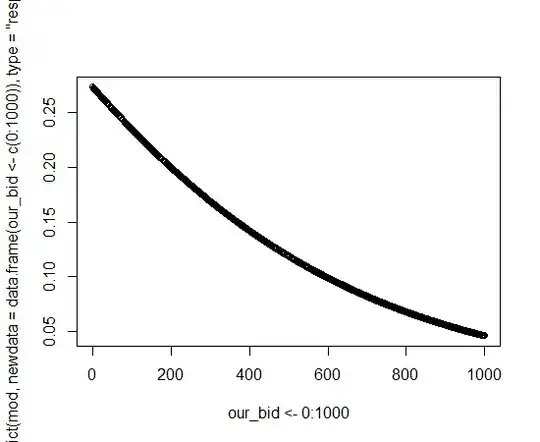
> plot(our_bid<-000:1000, predict(mod, newdata=data.frame(our_bid<-c(000:1000)),
       type="response"))

enter image description here

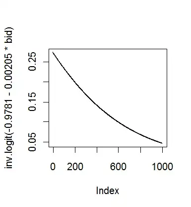
How can I go from this probability curve to an equation in R? I was hoping for something like:

Probability = -0.08*bid3 + 0.0364*bid2 - 0.0281*bid + 4E-14
gung - Reinstate Monica
  • 132,789
  • 81
  • 357
  • 650
ATMathew
  • 2,165
  • 11
  • 28
  • 42
  • 2
    Unlike the example in your code, which has *one* independent variable (bid) and therefore plots as a curve in a (bid, probability) plane, the example in your edit at the end would not plot as a curve: it would be a *three* -dimensional hypersurface plotted in four dimensions (bid, bid2, bid3, probability). – whuber Jan 09 '12 at 18:51

1 Answers1

15

This generalized linear model supposes the outcome associated with an independent value of $x$ has a binomial distribution whose log odds ("logit") vary linearly with $x$. The output provides the coefficients of that linear relation; namely, the intercept is estimated as -0.9781 and the slope ("our_bid") as -0.002050. You can see them in the Estimate column:

              Estimate Std. Error z value Pr(>|z|)    
(Intercept) -9.781e-01  2.836e-02  -34.49   <2e-16 ***
our_bid     -2.050e-03  7.576e-05  -27.07   <2e-16 ***

The probability, which you wish to plot, is related to the log odds by

$$\text{probability} = \frac{1}{1 + \exp(-\text{log odds})}.$$

R calls this the "inverse logit" function, inv.logit.

Putting these together gives the equation

$$\text{probability} = \frac{1}{1 + \exp\left(-[-0.9781 - 0.00205 x]\right)}.$$

An R command to plot it would be

plot(inv.logit(-0.9781 - 0.00205*(0:1000)))

Plot output

In general, you should extract these coefficients with the coefficients command rather than transcribing them (as I did here, because I do not have access to your data).

whuber
  • 281,159
  • 54
  • 637
  • 1,101
  • 3
    (+1) Of note, the `Hmisc::latex` function makes it easy to print the above as $\LaTeX$, e.g. `latex(fit.1)` may yield [this output](http://i.imgur.com/7FlMr.png) (using [sample code here](http://stats.stackexchange.com/a/9808/930)). – chl Jan 09 '12 at 19:44