Plots of residuals in linear regression

Question

I wanted to know the intuition behind the plots of residuals vs time, residuals vs fitted values and residuals vs explanatory variables.

Could anyone intuitively explain to me what they are supposed to indicate in case they are not random (which I am told, is the way we want these plots to be)

Also, are there any other residual plots used in the diagnostics of linear regression that I am missing here?

Answer 1

So, which ways can we helpfully plot residuals in linear regression? There are many, so let us go through them.

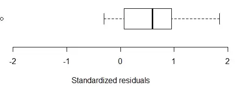
1. QQplots of residuals, that is, quantile-quantile plots. This is usually used to compare the distribution of residuals to the normal distribution, although it could be used also to compare to some other theoretical distribution. There are many answered Qs on this site, some: How to interpret this QQ plot? How to interpret qq plot "not on the line"? How to interpret a QQ plot One can also make confidence bands on the QQ plot, see Confidence bands for QQ line

2. One assumption in linear regression is homoskedasticity, that is, constant variance. That can be checked graphically by plotting residuals against fitted values. Examples and discussion in What does having "constant variance" in a linear regression model mean? (the plot residuals versus fitted could also show some kinds of unmodeled nonlinearity)

3. Some standard plots produced (in R) by plot(some.lm.object) is discussed in Interpreting plot.lm()

4. It can be useful to plot residuals against individual predictors. Let us look at some examples. I will use the minitab tree data contained in R:

   data(trees)
   colnames(trees)
   [1] "Girth"  "Height" "Volume"
   

We will build a linear model for Volume with predictors Girth and Height. We know that doesn't make sense, as volume should be the product and not the sum! That way, the example is good to see if we can detect this model error from residual plots.

mod1  <-  lm(Volume ~ Girth + Height, data=trees)

The plot of residuals versus Girth:

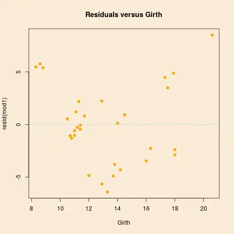
We added a horizontal reference line at zero. If the model is adequate, the residuals should spread randomly around this line. Here we can clearly see a "U" form, indicating unmodeled nonlinearity, that is, the effect of Girth on Volume is not linear as modeled. The similar plot for Height is less clear (not shown).

Now, if we use some knowledge of the geometry of trees, and model a tree as a cylinder or a cone, the formula for colume will have the form $$ \text{Volume} = C\cdot \text{Girth}\cdot \text{Height} $$ (where the constant $C$ will have different values for "cylinder", "cone" or "truncated cone"). Taking logarithms we get $$ \log(\text{Volume}) = \log(C) + \log(\text{Girth}) + \log(\text{Height}) $$ which can be estimated as linear model:

mod2  <-  lm( log(Volume) ~ log(Girth) + log(Height),  data=trees)
> summary(mod2)

Call:
lm(formula = log(Volume) ~ log(Girth) + log(Height), data = trees)

Residuals:
      Min        1Q    Median        3Q       Max 
-0.168561 -0.048488  0.002431  0.063637  0.129223 

Coefficients:
            Estimate Std. Error t value Pr(>|t|)    
(Intercept) -6.63162    0.79979  -8.292 5.06e-09 ***
log(Girth)   1.98265    0.07501  26.432  < 2e-16 ***
log(Height)  1.11712    0.20444   5.464 7.81e-06 ***
---
Signif. codes:  0 ‘***’ 0.001 ‘**’ 0.01 ‘*’ 0.05 ‘.’ 0.1 ‘ ’ 1

Residual standard error: 0.08139 on 28 degrees of freedom
Multiple R-squared:  0.9777,    Adjusted R-squared:  0.9761 
F-statistic: 613.2 on 2 and 28 DF,  p-value: < 2.2e-16

and note that now actually the coefficient estimates makes geometrical sense! Is the residual plot any better?